A Primer on Search Algorithms

“It’s written, ‘seek and ye shall find’. But first, ‘imagine what you seek’. Otherwise, you will end up searching everything everywhere forever.” Toba Beta, My Ancestor Was an Ancient Astronaut
This article will be a primer on search algorithms used in Artificial Intelligence. This article was formed from lecture notes from COMP111 at the University of Liverpool taught by Frank Wolter and the famous Russel, Norvig book Artificial Intelligence: A Modern Approach.
Uninformed Search Strategies
An uninformed search strategy has no information about states beyond what is the goal state, what is not the goal state and what are the successor states.
Breadth first search
Breadth First Search (BFS) is a search algorithm developed by Konrad Zeus for his rejected PhD thesis in 1945. Breadth First Search searches all neighbors before it searches child nodes. In the below picture, once the start state (1) has been searched the states 2, 3, and 4 will then be searched.
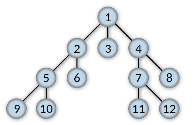
The Breadth First Search Algorithm has a queue which is vital to how it works. Breadth first will first check whether the current node it is searching is the goal state or not. If it is not the goal state, it places all child nodes of the current node being searched into a queue. If 2 is being searched then the queue will look like [5, 6, 3, 4].
Because of the first in first out nature, the first ones added to the queue are the first ones out of the queue, so it would search in the order 4, 3, 6, 5.
There is also a second list, a list of every node that has already been visited in the search tree.
Advantages
Breadth-first search is complete. It will always find a path and the shortest path to the goal, assuming the goal is at a finite depth.
Disadvantages
Consider a theoretical state where every state has b successors. The root of the search tree generates b nodes and the second level of the search tree generates b² nodes. Each level generates b more nodes, yielding b^n (b to the power of n) nodes where n is the level the search tree is on.
Now suppose the goal is at depth d. In the worst possible case (computer scientists prefer to use worst possible cases instead of best or mediocre case) we would expand all but the last, goal node at level d (since the goal itself is not expanded) resulting in b^d+1 — b nodes at level d + 1. The total number of nodes explored is
b + b² + b³ + … b^d = O(b^d-1).
Note the above equation, O(b^d-1) is using Big O notation.
The -1 is because you do not explore the goal node, so the goal is at depth level -1.
The total number of nodes in the frontier is O(b^d), this is the space complexity.
Every node must stay in memory because it is either apart of the frontier or an ancestor of the frontier. The space complexity is therefore the same as the time complexity.
Time and Space complexity
Time complexity is how long it takes the algorithm to run given an input, usually denoted in Big O notation. Space complexity is how much the algorithm takes up in memory. Although this depends on the hardware factors, just like with Big O notation we can use a notation to represent how much space it’ll take up.
In the above example, Breadth First Search takes an enormous amount of time and space complexity.
Uniform Cost Search
A Gif demonstrating Dijkstra’s algorithm, similar to Uniform Cost Search Uniform Cost search is Dijkstra’s Algorithm but rather than finding the single shortest path to every point in the search tree it finds the single shortest path to the goal node.
Breathd first search is only optimal when all steps cost the same, because it always expands the shallowest unexpanded node. With a simple extension to breadth first search we can create an algorithm that is optimal for any cost. Instead of expanding the shallowest node like with BFS it instead expands the node, n, with the lowest path cost.
If all steps cost the same then Uniform Cost Search is identical to BFS.
Uniform cost search does not care about the number of steps a path has but instead it cares about their total cost. Therefore it is possible for BFS and Uniform Cost Search to get stuck in an infinite loop if it ever expands a node that has zero-cost leading back to the same state.
In other words, if Uniform Cost Search expands into a node with a cost path of zero from a node with a cost path of zero and there are two routes to each other it can get stuck in an infinite loop.
We can gurantee completeness using this search method by making sure the cost of every step is greater than or equal to a small positive constant.
Uniform Cost Search is guided by path costs and not lengths so it’s complexity cannot easily be shown. Instead, let X be the cost of the optimal solution and assume that every action costs at least Y. Then the algorithms worst case scenario is O(b[X/Y]) which can be much greater than B^d, which makes Uniform Cost Search slower and more resource hungry than Breadth First Search.
Depth First Search
Depth First Search expands the deepest node in the current frontier first. Depth first search goes immedtially to the deepest possible point of the search tree until there are no sucessors.
In this example, Depth First Search will go straight to 9, then 10 and then to 6.
Whereas Breadth First search uses a first in first out (FIFO) queue Depth First uses a a Last in Last out queue (LIFO). A LIFI queue means that the most recently generated node is chosen for expansion. The most recently generated node must be the deepest possible unexpanded node because it is deeper than its parent node.
If Depth First Sreach is used on a graph which avoids repeated states and redundant paths then it will find its goal in a finite number of states. If however it is used on a search tree then it will expand forever, in other words depth first search is not complete within search trees.
Depth first search will not find the optimal path.
The time complexity of DFS is 1+ b² + b³ + … +b^m
The advantage of DFS over BFS is the space complexity. Once a path has been fully explored it can be removed from memory, so DFS only needs to store the root node, all the children of the root node and where it currently is. DFS requires space complexity of O(bm)
Depth Limited Search
Depth Limited Search is a vartion on DFS whereby a limit is set to the depth of DFS so it does not go on forever or too long. It also solves the infinite path problem.
If the goal is at level N and we choose a depth of D and D < N then Depth Limited Search is incomplete.
The solution found is not guranteed to be the shortest optimal path.
The time complexity of Depth Limited Search is B^d where d is the depth limit.
The space complexity of depth limited search is B*d where d is the depth limit.
Iterative Deepening Depth First Search
Iterative deepning is a varation on Depth Limited Search whereby the depth limit is increased if the goal is not found. Iterative Deepning often starts at level 0 and then increases by a singular level if the goal isn’t found on that level.
Iterative Deepning Depth First Search combinds the best parts of depth-first search and breadth first search.
Iterative Deepning’s memory requirements are small, O(bd) where b is the amount of nodes generated and d is the depth level.
Iterative deepening may seem wasteful because nodes are generated multiple times, although this is not very costly. Consider a search tree with the same branching factor at each level; most of the nodes will be on the bottom level so it does not matter much to generate upper level nodes repeatedly.
In iterative deepning, nodes on the bottom level are generated once, those on the next to bottom level are generated twice and so on up to the children of the root node, which are generated d times. The total number of nodes generated are:
N(IDS) = d(b) + (d-1)b²+…+(1)b^d
Which gives us a time complexity of O(b^d)
Note the time complexity of breadth-first search given the same search tree:
N(BFS) = b + b² + … + b^d + (b^d+1 — b)
The result is that Iterative Deepening is faster than BFS although Frank says that it is slower but it uses alot less memory than BFS.
Bidirectional Search
The idea of bidrectional search is to run two searches, one forward from the start state and one backward from the goal state, stopping when the two searches meet. The idea is that b^d/2 + b^d/2 is much smaller than b^d.
Bidirectional search works by having one or both of the searches check the next node to see if it is in the fringe (frontier) of the other search tree, if it is then a solution has been found.
The time complexity of Bidirectional search is O(B^d/2)
Bidirectional search must be able to calculate the predecessors of states and must also know where the goal is.
Informed (Heuristic) Search Strategies
An informed search stratergy is one that uses problem-specific knowledge to find solutions more efficiently than an uninformed search strartergy.
Greedy Best-First Search
Greedy attempts to expand the node that is closet to the goal on the idea that it is likely to lead to a solution quickly.
It uses heuristics to determine which nodes are ‘closet’ to the goal node.
Greedy search is like depth first search in that it prefers to take a singular route to the goal and will back up when it hits a dead end. Greedy search is not optimal and it is incomplete because it can get stuck within an infinite loop.
The worst case time complexity of greedy search is O(b^m) where b is the amount of nodes and m is the maximum depth of the search space.
A* Search
The most widely known form of search algorihm is A* (a-star). It chooses its path based on 2 statistics, g(n) and h(n). g(n) is the cost to reach the node and h(n) is the heuristic function that shows the cost from the node to the goal.
f(n) = g(n) + h(n)
Provided that the heuristic function satisfies certain conditions then A* is both optimal and complete.
A* is optimal if h(n) is an **admissable heuristic**. That is provided that h(n) does not over estimate the cost to reach the goal. Admissable heuristics are often optimistic as they think the cost of solving the problem is less than it actually is. Since g(n) is the exact cost to reach n, we have an immedtiate consequence that f(n) never overestimates the true cost of a solution through n.
A* is normally not suitable for large search problems.
Games vs Search Problems
In traditional search algorithms the user makes all the moves, however in a game we implement search algorithms against an unpredictable enemy.
The best possible way is to calcualate every single possible move the enemy can make and counter them, although this will cause a combinatoral explosion in which the computer will take too long to calculate the correct answer.
In reality, we need to use heuristics to calculate search problems in games.
In some games we have a fully observable environment, we know everything about the environment such as Chess or Go. In other games we have partial information where we don’t fully know the environment, such as Poker.
Minimax algorithm
In a game, Min and Max are two players. Max wants to win (maximise the utility of each move) whereas Min wants Max to lose (minimise utility for max).
The game Minimax is used on has to be a zero sum game, that means that there can only be winners and losers, nothing in between; like Chess.
The set of goal states is replaced by a utility function.
Max wants a strategy for maximising utility assuming min will do the best it can to minimise max’s utility.
The utility of a MAX-state (where Max moves) is the maximum of the utilities of its successor states.
The utility of a MIN-state (where Min moves) is the maximum of the utilities of its successor state.
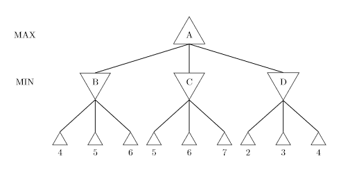
Taken from University of Liverpool homework The Minimax starts from the bottom, with Min (player 1) starting first. You know min starts first because it is denoted in the left hand side. Min would choose the lowest possible value, so for level 1 it would be {4, 5, 2} since these are the lowest possible values in the tree.
We then move one level up. The Minimax values of A is the maximum value of {4, 5, 2} which is 5. So Max would choose 5.
In game playing, minimum would want Max to choose the one with the lowest utility, as a higher utility might attack or hurt player 1 more than a lower utility.
In a game such as chess the trees are extremely large. In chess the number of moves grow exponentially, after 4 moves there are 288 billion different possible positions. This is where Alpha-Beta pruning comes in. We cut off large chunks of the tree that we believe we no longer need in order to allow the Minimax algorithm to run in efficient time, that is time that will take less than 10 minutes to run (roughly).
Minimax tries to reduce the maximum damage the opponent can do whilest reaping the maximum possible reward for us assuming the opponent plays optimally.