Absolute Fundamentals of Artificial Intelligence


Machine learning, what a buzzword. I’m sure you all want to understand machine learning, and that’s what I’m going to teach in this article.
I found that learning the theroetical side alongside the programming side makes it easier to learn both, so this article features both easy to understand mathematics and the algorithms implemented in Python. Also, technology becomes outdated — fast. The code used in this tutorial will likely be meaningless in 5 years time. So for that reason, I’ve decided to also teach the mathematical side to Machine Learning that will not die out in a few years.
What is machine learning?
Let’s start with learning. Learning is a long and complicated process to describe but in a nutshell it is turning experience into knowledge.
Machine learning is teaching machines how to learn, as insane as that sounds it’s actually plausable using probability.
I highly reccomend you read this article on probability, as it is the essential foundation to machine learning and artifical intelligence. We will go over conditional probability and Bayes therom again in this article.
Types of learning
There are many different ways for a machine to learn, in this I try to explain the different types.
Supervised Learning
In supervised learning we start with a dataset that has training examples, each example has an assiocated label which identifies it.
An example of this is presented below:
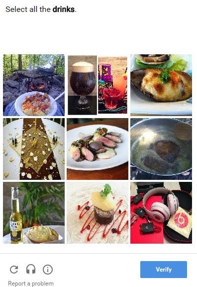
Google ReCaptcha We want the machine to be able to identify drinks, so we present the machine with 9 images, some containing drinks. We then select the pictures that contains the drinks, teaching the computer what a drink looks like.
It does this by running labelled data through a **learning algorithm. **The goal of supervised learning is to be able to correctly identify new data given to it, having learnt how to identify the data using the previous data set and learning algorithm.
Unsupervised Learning
Unsupervised learning is quite different from supervised in the sense that it almost always does not have a definite output. The learning agent aims to find structures or patterns in the data.
A good article on unsupervised learning can be found here.
Reinforcement Learning
Reinforcement learning is where the learner receives rewards and punishments for its actions. The reward could simply be utility and the agent could be told to receive as much utility as possible in order to “win”. Utility here could just be a normal variable.
A good example of reinforcement learning is this:
Machine Learning
Now we understand some of the terminiology of machine learning, we’re actually going to teach a machine something. In order for us to do that, we need to learn a bit of probability.
Most of the probability here is directly copied off of another blogpost I wrote on probability, but I’ll only include the important parts required for machine learning here.
Conditional Probability
Conditional probability is where an event can only happen if another event has happened. Let’s start with an easy problem:
John’s favourite programming languages are Haskell and x86 Assembley. Let A represent the event that he forces a class to learn Haskell and B represent the event that he forces a class to learn x86 Assembley.On a randomly selected day, John is taken over by Satan himself, so the probability of P(A) is 0.6 and the probability of P(B) is 0.4 and the conditional probability that he teaches Haskell, given that he has taught x86 Assembley that day is P(A|B) = 0.7.Based on the information, what is P(B|A), the conditional probability that John teaches x86 Assembley given that he taught Haskell, rounded to the nearest hundredth?
Therefore the probability of P(A and B) = P(A|B) * P(B); read “|” as given, as in, “A|B” is read as “A given B”. It can also be written as P(B|A) * P(A).
The reason it is P(A|B) * P(B) is because given the probability of “Given the probability that B happens, A happens” and the probability of B asP(B). (A|B) is a different probability to P(B) and P(A and B) can only happen if P(B) happens which then allows P(B|A) to happen.
So we can transform this into a mathematical formula:
P(A and B) = P(A|B) * P(B) = 0.7 * 0.5 = 0.35Solving it P(B|A) * P(A) P(A) = 0.5 So 0.6 * P(B|A) Now we don’t know what P(B|A) is, but we want to find out. We know that P(B|A) must be a part of P(A and B) because P(A and B) is the probability that both of these events happen so…P(A and B) = 0.350.35 = P(B|A) * 0.5 With simple algebraic manipulation 0.35/0.5 = P(B|A) P(B|A) = 0.7
Bayes Therom
Bayes Therom allows us to work out the probability of events given prior knowledge about the events. It is more of an observation than a therom, as it correctly works all the time. Bayes therom is created by Thomas Bayes, who noted this observation in a notebook. He never published it, so he wasn’t recgonised for his famous therom during his life time.
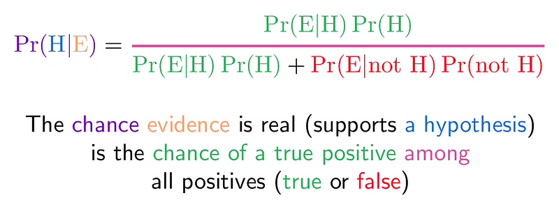
From https://betterexplained.com/articles/colorized-math-equations/ Confusing, right? Let us look at an example.
Suppose a new drug is found on the streets and the police want to identify whether someone is a user or not.The drug is 99% sensitive, that is that the proportion of people who are correctly identified as taking the drug.The drug is 99% specific, that is that the proportion of people who are correctly identified as not taking the drug.Note: there is a 1% false positive rate for both users and non users.Suppose that 0.5% of people at John Moores (A rival university) takes the drug. What is the probability that a randomly selected John Moores student with a positive test is a user?
Let’s colourfy this and put this into the equation
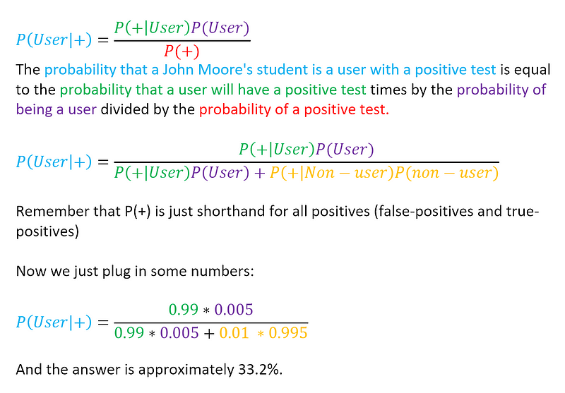
Note: we don’t directly know the chance of a positive test actually being positive, it isn’t given to us so we have to calculate it, that is why the formula expands on the denominator in the second part.
Learning with Bayes Therom
Now, bayes therom isn’t designed to be used only once. It is designed to work with continus data. Baye originally created this using a thought experiment. He wondered that if his assistant threw a ball on the table, can he predict where it will land?
Baye asked his assistant to do just that. Then again, and to tell him whether it was left or right of the original spot. He noted down every single spot it hit, and over time, with each throw, he got better at predicting where it’ll land. This is where bayes therom comes into play, by repeatedly using bayes therom we can overtime calculate where the ball might land more accurcately.
Let’s do a quick example just to get some numbers:

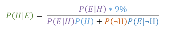
Medium doesn’t support colours, so I have to copy and paste images. Sorry! So what would happen if you went to another hospital, got a second opinion and had the test run again by a different lab? This test also comes back as positive, so what is the probability you have the disease?
We change the postieor probability of having the disease before the test to 9%, so it looks like this:
Now the new number is 0.9073319 or 91% chance of having the disease.
Which makes sense, 2 positive results from 2 different labs are unlikely to be conincidental. And if you get more lab results done and they all come back as positive, this number will gradually increase towards 100%.
Naive Bayes Classifier
Naive Bayes Classifier is a type of classifier that is based on Bayes’ Therom with an assumption of independence among predictors. A Naive Bayes Classifier assumes that the presence of a particular feature is unrelated to the presence of any other feature. For example, a frut may be considered an apple if it is red, round, and about 3 inches in diameter. Even if these features depend on each other or upon the existance of all other features of an apple, all of these contribute to the probability that the fruit is an apple and that is why this classifier is known “ Naive”.
Wikipedia put it nicely:
In simple terms, a naive Bayes classifier assumes that the presence (or absence) of a particular feature of a class is unrelated to the presence (or absence) of any other feature, given the class variable. For example, a fruit may be considered to be an apple if it is red, round, and about 4” in diameter. Even if these features depend on each other or upon the existence of the other features, a naive Bayes classifier considers all of these properties to independently contribute to the probability that this fruit is an apple.
Problem
Suppose we have 2 datasets, “play” and “weather”. We want to see the possibillities of playing given the weather.
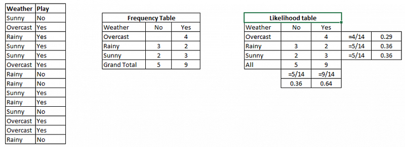
Image from https://www.analyticsvidhya.com/blog/2017/09/naive-bayes-explained/
- The first step is to turn the data into a frequency table
- The second step is to create a likelihood table by finding the probabilities like Overcast = 0.29 and the probability of playing is 4 / 14 (where 14 is the amount of times they play overall) and 4 is the number of times they played in that weather previously.
- Now use the Naieve Bayesian equation to calculate the conditional probability for each class.
Here’s an example problem question solved using the above data and the equation.
Is the statement “players will play if weather is sunny” correct?
P(Yes | Sunny) = P(Sunny|Yes) * P(Yes) /P(Sunny)
Remember Bayes Therom? This is the same but with variable names inputted to make it easier to read.
Now we have P(Sunny|Yes) = 3/9 = 0.33. P(Sunny) = 5/14 = 0.36. P(yes) = 9/14 = 0.64Now using Bayes Therom we can work out P(Yes|Sunny) = 0.33 * 0.674 / 0.36 = 0.60 which has high probability.Thus, given that it is sunny, there is a 60% chance they will play.
Machine Learning using Python
Wow, what a boring read that was. “Theoretical Computer Science is boring” I hear you say. Well, you’ll be excited to know this next part is about the application of machine learning using Python.
Let’s calculate whether an email is spam or ham (that is, a normal email) using machine learning.
So, given a large corpus of ham and spam emails, we need to train the model. We’ll start by calculating for each word in each email the number of times that word appears in spam and ham emails.
We’ll then calculate a “spaminess” level of each word using a formula. The formula we will be using is quite simple.
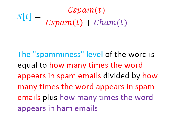
So, the numerator (the number on top) shows how many times the word appears in a spam email, and the denominator (the bottom) shows how many times it appears in any email.
So, lets say there are 9 spam emails and 10 ham emails, making 19 total. If a word appears in 9 spam emails, but 1 ham email than the equation is 9/10 which gives us a 90% chance that this word means it is a spam email.
But we cannot simply just count one word, we need to do this for all the words in the email.
We essentially have 3 steps:
- Find the spamminess of each word in a message.
- Find the total spamminess of a message, say by multiplying together the spaminess levels of each word. Call this S[M].
- Then find the haminess of each word, by multiplying together the (1 — spaminess) level of each word. Call this H[M].
Then if S[M] > H[M] then the message is spam, else it is ham.
Okay, so let’s implement this. We’ll be using the bodies of emails only, and there won’t be many emails just to make the explanation easy. Also, the spam emails are **fairly **obvious. Below is the bad emails text file I’m using
Viagra for sale, get sexy body soon! U want sum viagra bby? u sexy s00n VIAGRA VIAGRA VIAGRA VIAGRA VIAGRA SEXY SOON VIAGRA PLEASE YASSSSS VIAGRA BUY PLEASE I really like today
And the good emails
Hello, how are you? I hope you have the work ready for January the 8th. Do you like cats or dogs? Viagra viagra
So the first step is to somehow take this file and split it up.
The code reads the file, and splits it per new line, spitting out 2 lists. The lists look like this. Below is the bad emails
[‘Viagra for sale, get sexy body soon!', ‘U want sum viagra bby? u sexy s00n’, ‘VIAGRA VIAGRA VIAGRA VIAGRA VIAGRA’, ‘SEXY SOON VIAGRA PLEASE YASSSSS ‘, ‘VIAGRA BUY PLEASE’, ‘I really like today’]
And the good emails
[‘Hello, how are you?', ‘I hope you have the work ready for January the 8th.', ‘Do you like cats or dogs?', ‘Viagra’, ‘viagra’]
Okay, now we need to calculate the spaminess of each word. We do this by finding the word, and seeing how many times it appears in the bad emails and how many times it appears in the good emails, basically the formula seen here:
So to find out how many words appear in bad and good emails, we could use nested for loops; but I’ve opted to go a bit functional here.
So, the first line is a lambda (anonymous) function which just turns a list of lists into one list. Anonymous functions are functions that are only intended to be used once or twice. The second and third line do the same. First, they map the function “x.split(“ “)” onto each email in the list, generating a new list of list of words in the email, then they apply the flatten function to make the list of lists into one list.
Now we have 2 lists, one containing all the words in a bad email and one containing all the good words in a good email.
Now we create a function that calculates the spamminess level of a word. First, it counts how many times a word appears in the bad emails. Then it counts how many times it appears in both emails. Then it returns how many times it appears in bad emails divided by how many times it appears in total emails.
Now we want a dictionary of every word and its spaminess level.
word_Dict shall now return
{‘body’: 1.0, ‘': 1.0, ‘want’: 1.0, ‘get’: 1.0, ‘I’: 0.5, ‘January’: 0.0, ‘s00n’: 1.0, ‘SOON’: 1.0, ‘you?': 0.0, ‘dogs?': 0.0, ‘sale,': 1.0, ‘U’: 1.0, ‘are’: 0.0, ‘Viagra’: 0.5, ‘sexy’: 1.0, ‘ready’: 0.0, ‘SEXY’: 1.0, ‘the’: 0.0, ‘8th.': 0.0, ‘really’: 1.0, ‘Do’: 0.0, ‘Hello,': 0.0, ‘BUY’: 1.0, ‘bby?': 1.0, ‘like’: 0.5, ‘for’: 0.5, ‘sum’: 1.0, ‘work’: 0.0, ‘PLEASE’: 1.0, ‘VIAGRA’: 1.0, ‘YASSSSS’: 1.0, ‘how’: 0.0, ‘viagra’: 0.5, ‘cats’: 0.0, ‘u’: 1.0, ‘hope’: 0.0, ‘have’: 0.0, ‘you’: 0.0, ‘or’: 0.0, ‘today’: 1.0, ‘soon!': 1.0}
Given a message, this code will compute how spammy the message is by multiplying the spaminess level of each word. The reduce function is foldl in haskell, it takes a list and a function and returns a single value by applying the function to every item of the list. In this case, given a list of [x, y, x, y, x, y] it will multiply x*y and then add that together.
Now we need to find the haminess of each message, not so hard now that we can find the spaminess.
The haminess is 1 — the spaminess
Now we just need to create a function that determines whether it is spam or ham.
If it is true, it is spam, if not; it’s ham. Obviously this won’t work so well with such a limited dataset, but if we had thousands of emails this should work well, despite the initial startup time being slow.
We just used a naieve bayes classifer — a supervised machine learning based approach to spam detection. Isn’t that really cool sounding?
K-Nearest Neighbour
Like Naieve Bayes above, let’s create an intution about K-nearest neighbour.
Let’s start off with some facts to build up this intuition.
A point is a location. It has no size, but much like any location it shows you where something is. It can be represented in different ways, depending on how many dimensions it lives in.
A line is a 1 dimensional object. We can represent a location on a line like so
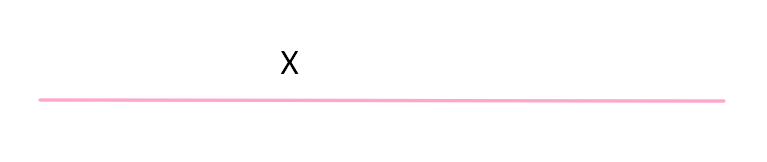
So say the line starts at the number 3 and ends at the number 9, a location is any number between 3 and 9. In this diagram, it is represented as X.
In a 2-dimensional object such as a square, we can represent the location using X and Y coordinates.
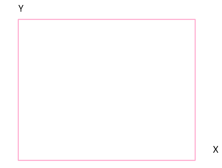
Any location in this square can be reached using X and Y coordinatess.
A cube is a 3-dimensional square, we can represent its location using 3 coordinates
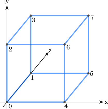
Taken from here A point in geometry is a location. It has no size i.e. no width, no length and no depth. A point is shown by a dot.
So a point in an n-dimensional space needs n coordinates to represent it. We find it hard to visualise anything more than 3 dimensional space (as our world is 3 dimensional).
An n-dimensional space is represented by an n-dimensional hypercube.
A hypercube is just a fancy word meaning that any location can be represented as a tuple of n numbers.
Now, back to the example of stopping spam. Any email message can be represented as a point in a hypercube.
Let’s say for example, we have a list of every single possible word that could ever appear in an email.
So there are:
W1, W2, …, Wn
Words in the list. Let’s simplfy this, lets say every single word that could appear in an email is
(‘Hello’, ‘Goodbye’, ‘Email’, ‘Cheese’, ‘United Kingdom’)
for simplicities sake, we’ll pretend only these words are possible in an email.
Every single email will contain a subset of the words above like so:
“Hello, Cheese.” or “United Kingdom, Goodbye.”
Each of these messages can be represented as a list of 1’s and 0’s, just like bit vectors.
So for the first message:
(‘Hello’, ‘Cheese’) (1, 0, 0, 1, 0)
So we simply turn the words that are in both the email and the universe of possible words into a 1, in this instance the first element, “Hello”, and the fouth element, “cheese” are turned into 1s.
So now we’ve taken a message and turned it into a point in an n-dimensional hypercube.
Now we want to do this for the email we want to classify as well as every email we hold information about. So we have training data, and a message to classify.
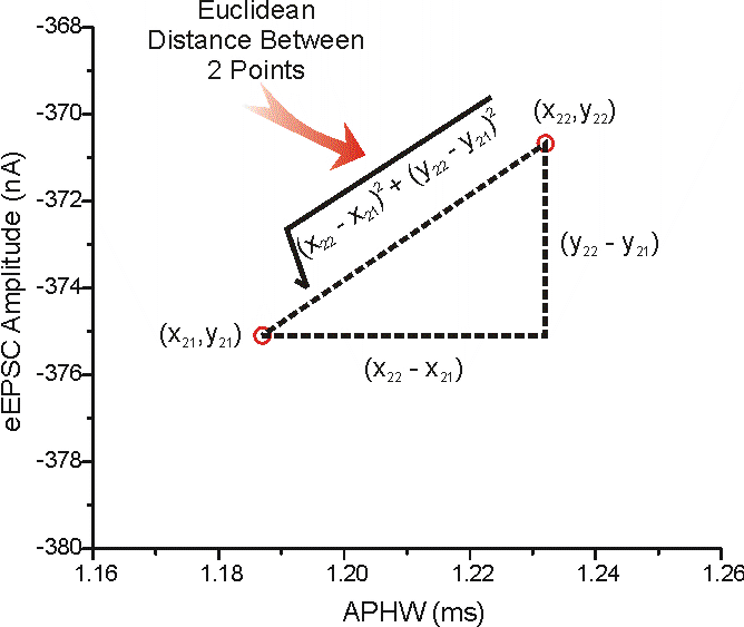
Now we have a bunch of points in an n-dimensional hypercube, we want to calculate the distance between each point. There are many ways to calculate the distance. We’ll be using the Euclidean Distance Formula here.

Taken from here. More on this later. When we insert a new email to be classified, we check its nearest neighbours. If most of the emails near it are spam, then the email is likely to be spam. But if most of the emails near it are ham, then the email is likely to be ham.
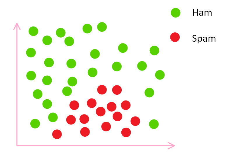
The feature space for spam and ham emails So we have our training data classified and this is what it looks like on a graph. When we place our email to be classified into it, the graph will look like:
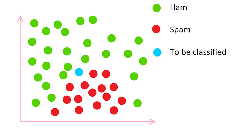
Feature space We know where to place the email to be classified because we turned it into a set of coordinates earlier.
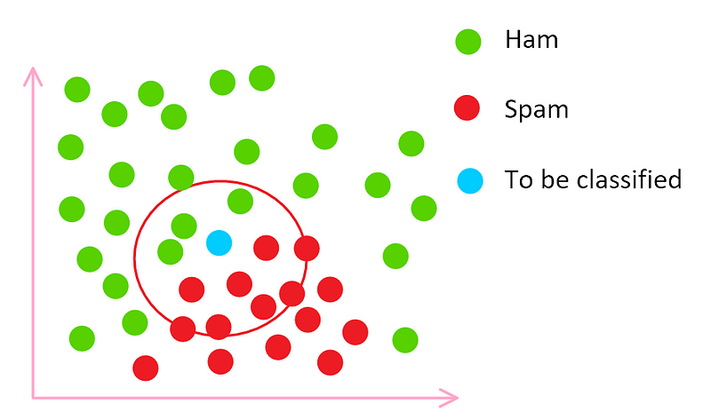
Feature space We draw a circle around the email to be classified and since most of the spam emails are inside the circle, we mark this email as spam. This is slightly simpler than reality.
When we categorised each email as a bit vector containing 0 and 1s, normally we would hash subsets of the email and use that instead and the distance will likely not be a straight euclidean formula but a more sophisticated formula that works well in training.
Distance Measurements
I said that Euclidean Distance was one of the ways you could calculate the distance, in this section I’m going to talk a little more about that.
The Euclidean Distance is used for **quantitative **data, data that is only numbers.
What is “Euclidean Distance”?
Well, first let’s go back to Pythagoras’ Therom. We all remember it as
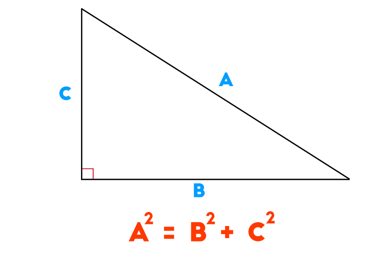
Taken from here but Pythagoras’ therom can be applied to many instances. In short, it is findign the distance between 2 points at a right angle. Let’s say you walk 3 meters east and 4 meters north, how far away are you from the original source? Well, 5 meters as the crow flies. If you want to learn more about how the Pythagoras’ Formula can be used to find any distance, read this article:
How To Measure Any Distance With The Pythagorean Theorem *We’ve underestimated the Pythagorean theorem all along. It’s not about triangles; it can apply to any shape. It’s not…*betterexplained.com
The actual formual for euclidean distance is:
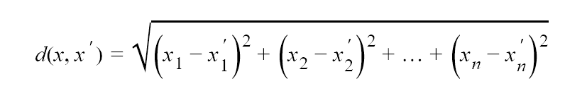
Notice how it’s very similar to Pythagoras’ therom.
Let’s say we have this table:
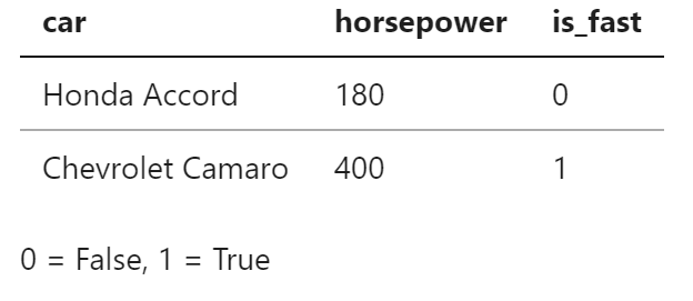
We want to find the distance between these 2 cars, so we insert the values into the Euclidean Distance formula as such:
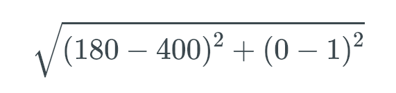
Thus the distance is around 220.
What About Qualitative Data?
Qualitative data is data that cannot be represented as a number. Let’s try an example:
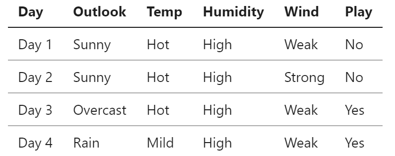
Table inspired by slides from Frank Wolter, AI Lectuer @ UoL Lets say you have data of the weather over 4 days and whether or not children in a school played during breaktime. There’s no numbers here, so we cannot use the Euclidean Distance. You cannot square a concept like “sunny” or squareroot the resultant concept.
So we have to find a different way of measuring how close a day is to another. Let’s take day 1 and day 3. How simialr are they? There is an equally natural way of doing this, we just count the number of features on which the days are the same.
So day 1 and 2 have all the same features apart from wind, so we give it a distance of 1. We count the amount of features that differ.
So day 1 and 3 have a distance of 2.
You can easily change this corresponding to what you believe is more important, this method isn’t a one size fits all method but rather a method that you, as a human being (and not AI; hopefully) need to decide on.
What defines an ‘neighbour’
You may have spotted something weird earlier that I didn’t expand on here:
Feature space How was the size of the circle decided? Well, good question. This is a very typical problem in learning. Do you want the nearest 3 neighbours or the nearest 20 neighbours? Well, that all depends on your training data. This is entirely down to you.
Implementing K Nearest Neighbour in Python
So now we understand K nearest neighbour, lets implement it in Python. Here is the data we’ll be using in Comma Seperated Value (CSV) format.
Note: This section uses code from here,here, and here.
Download the file here either by running the command
wget https://archive.ics.uci.edu/ml/machine-learning-databases/iris/iris.data
In a Terminal or by selecting all the lines on the website, copying them and pasting them into a text file called iris.data.
Next up we want to read in the data like so:
The csv module allows us to work with comma seperated value (CSV) files. If you were to print it by adding the following to the code
You would get something like this as an output, but much longer.
6.5, 3.2, 5.1, 2.0, Iris-virginica 6.4, 2.7, 5.3, 1.9, Iris-virginica 6.8, 3.0, 5.5, 2.1, Iris-virginica 5.7, 2.5, 5.0, 2.0, Iris-virginica 5.8, 2.8, 5.1, 2.4, Iris-virginica 6.4, 3.2, 5.3, 2.3, Iris-virginica
Now we need to make 2 datasets, one is a training dataset and the other is a test dataset. The training dataset is used to allow K-nearest neighbour (KNN) to make predictions (note: KNN does not *generalise *the data)
The file we just loaded was loaded in as strings, so we need to turm them into numbers we can work with then we need to split the data set randomly into training and testing datasets. A ratio of 2/3 for training and 1/3 for testing is normally the standard ratio used.
Note to the reader: I had a hard time trying to import the iris data on my own, so this code is exactly copied from here.
Now we want to calculate the Euclidean Distance between 2 points, since the flower dataset is mostly numbers and a small string at the end, we can just use the euclidean distance and ignore the final feature.
Woah! What is that? This is functional programming. I’ve just completed a 12-week functional programming class and as my lectuer said:
By the end of 12 weeks, you will be the person who always says “this could be done in 1 line in functional” to every bit of code you read
Let’s divert quickly from AI and have a run down over this functional code. With functional, it’s best to read inwards to outwards so we’ll start with the first functional bit of code
Note: the remove_flowers function will be talked about later, but without this here it causes an error in the code later on. remove_flowers just turns an item of data like
5.0,3.4,1.5,0.2,Iris-setosa
into
5.0,3.4,1.5,0.2
Map is a function which applies a function to every item in a list. The function it is applying is a lambda (anonymous) function. An lambda function is a function which is only used for one purpose, so it doesn’t need to have its own define statement. The syntax for a lambda looks like this:
Lambda var1, var2: calculation
In this instance we have 2 variables, x and y and we are putting them into Pythagoras’ Therom. The map syntax is:
map ( function, list)
But our map takes 2 lists, X and Y. When it does the maths, it takes the first element of list1 and makes it into a variable called x, then it takes the second element of list2 and makes it into a variable called y. it does this until all items in both lists are finished.
The last part, list, turns our map into a list. So we get a list containing the Pythagoras’ Therom output of every item in both list1 and list2, which is just
[4, 4, 4]
Our next piece of code is
Now we know what list(map(… does we can just ignore it and treat it as a function which returns [4, 4, 4].
So that leaves us with this funky function:
Now, reduce is just foldl from Haskell but implemented in Python. It takes a list and turns it into one single value. It does this by applying a function to a list. The function it is applying is again a lambda function, where it adds the x and y together. What are x and y? Say we have a list like so
[1, 2, 3]
then when we add x + y we get
[1, 2, 3] x = 1, y = 2 1 + 2 = 3 x = 3, y = 3 x + y = 6
Now, we know what the lambda function does inside reduce, what list is it applying to? Well, reduce is taking the list produced by our earlier map function and turning it into one value.
So list is taking [4, 4, 4] and just adding them together. 4 + 4 + 4 = 12. So the output is 12.
Now we just need to find the square root of it all, which is simple.
Although this may not be readable, it’s simple to understand once you know some functional programming.
There’s a slight error, the flowers all end with a string representing what flower it is. We can’t perform math on this, so we have to use this function
to any list we pass to the Euclidean Distance function.
Now we need to find the distance from every item in the training set to the item in the test set.
This code simply maps a lambda (anonymous) function onto every element in the training and test sets which finds the distance between the two elements and returns those distances in a list. The second part then zips together the element with the corresponding distance. So the first part returns
[3.4641016151377544, 0.0]
When given these parameters
trainSet = [[2, 2, 2, ‘a’], [4, 4, 4, ‘b’]]testInstance = [4, 4, 4]k = 1
and the second part returns this
[([2, 2, 2, ‘a’], 3.4641016151377544), ([4, 4, 4, ‘b’], 0.0)]
The last part to the code orders the code and returns K many neighbours, in this instance K = 1 so it just returns
[[4, 4, 4, ‘b’]]
Next we need to somehow vote on what K could be, now that we know its neighbours. We’ll create a voting system. Each neighbor will vote on its attribute (IE, what it is) and the majority vote will be taken as the prediction. So if the majority of its neighbours are of class “a” then the prediction will be of class “a”.
So this just goes through all the nearest neighbours and keeps a dictionary. The dictionary is just the flowername + how many times it appears. Each flower votes for their type into the dictionary, the dictionary is sorted so the most amount of vote appears in the first item in the dictionary and then the predicted flower is returned.
And that’s it. We’ve put together a K-Nearest Neighbours classifier. If you want to read more about implementing this algorithm I suggest reading this or this.
K-Nearest Neighbour vs Naieve Bayes
It’s entirely down to you when to implement KNN or Naieve Bayes. There are some advantages and disadvantages to both, so I’ll list them here:
K-Nearest Neighbour Advantages
- Simple but effective
- Only a single parameter, K, easily leanred by cross validation
K-Nearest Neighbour Disadvantages
- What does nearest mean? Need to define a distance measure
- Computational cost — Must store and search through the entire trainign set at test time.
Note: The Netflix progress prize winner was essentially K-Nearest Neighbour.
Naieve Bayes Advantages
- Very simple to implement
- Needs less training data
- Can generalise the data
Naieve Bayes Disadvantages
- Accuracy increases with the more data it has, so to get a 95% or higher accuracy you’ll need alot of data
- Strong Independence Assumptions
You should now have a firm foundation in machine learning. Instead of teaching you an algorithm that will very likely be replaced in 3 years, I decided to teach the fundamental mathematicals and theroy that define these algorithms and then show 2 of the most widely used algorithms that will likely be around for a while.