Graph Theory

If you want to learn a lot about Graph Theory, check out this article
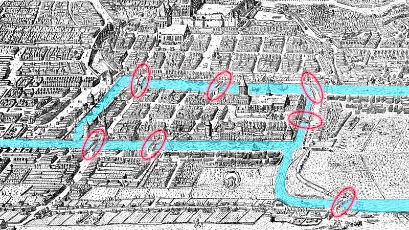
The seven bridges of Koenigsberg is the foundation and birth of graph theory.
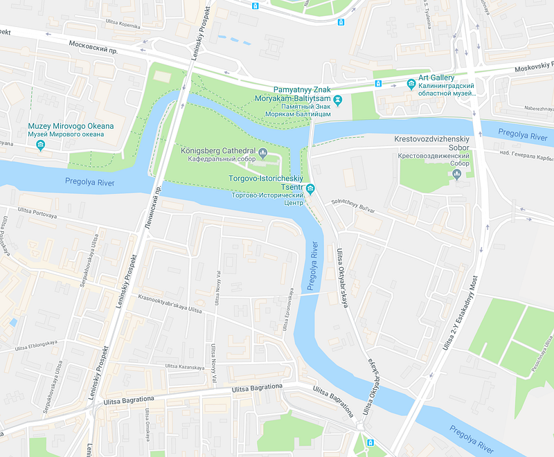
There was a puzzle that stated:
Can you cross all seven bridges exactly once?
There are 2 rules for this problem:
- Do not cross any bridge twice
- All bridges must be crossed
In the 18th Century a mathematician called Euler realised this problem was impossible. Every bit of land you enter has to have 2 bridges, or an even number of bridges. One you can leave on, one you can enter on.
You’ll notice a part of the land does not have an even number of bridges, it actually has 3 bridges.
Let’s move straight into graph theory.
An undirected graph G = (V, E) consists of a set of vertices V and a set of edges. It is an undirected graph because the edges do not have any direction.
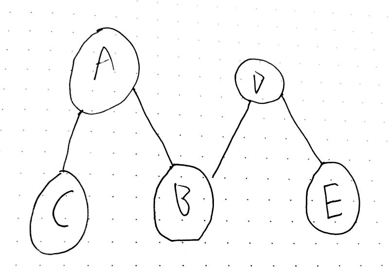
Each edge is an unordered pair of vertices. So {a, b} is the same as {b, a}.
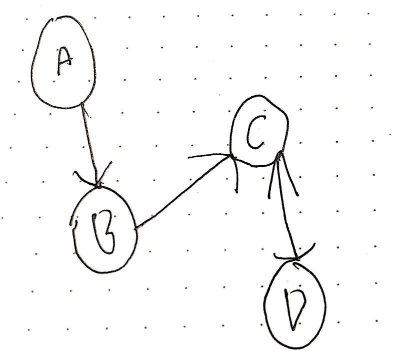
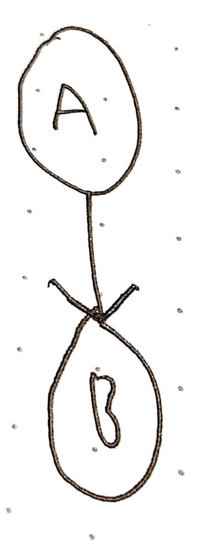
A directed graph G = (V, E) is where each vertex has a direction.
Think of it like Facebook and Twitter. On Facebook when you friend someone, the other person is automatically a friend of you.
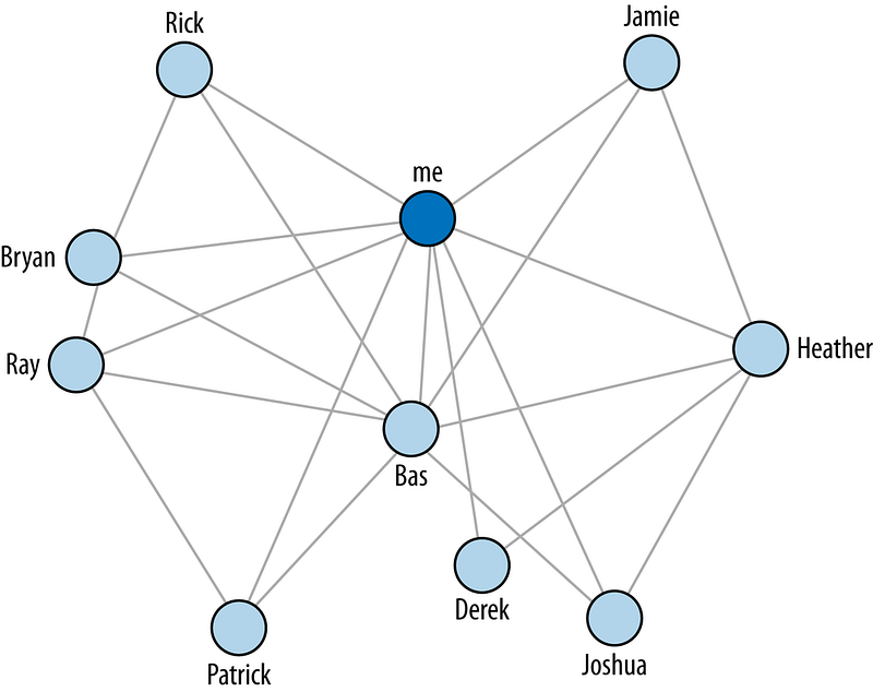
image from here
Graphs are used to model computer networks, state spaces of finite games such as Chess.
Here are some of the different types of graphs:
Simple Graph
The Simple Graph has at most 1 edge between 2 vertices and it has no self-loop. It has no edges that come from a vertex and go back to that same vertex.
This is not a simple graph:
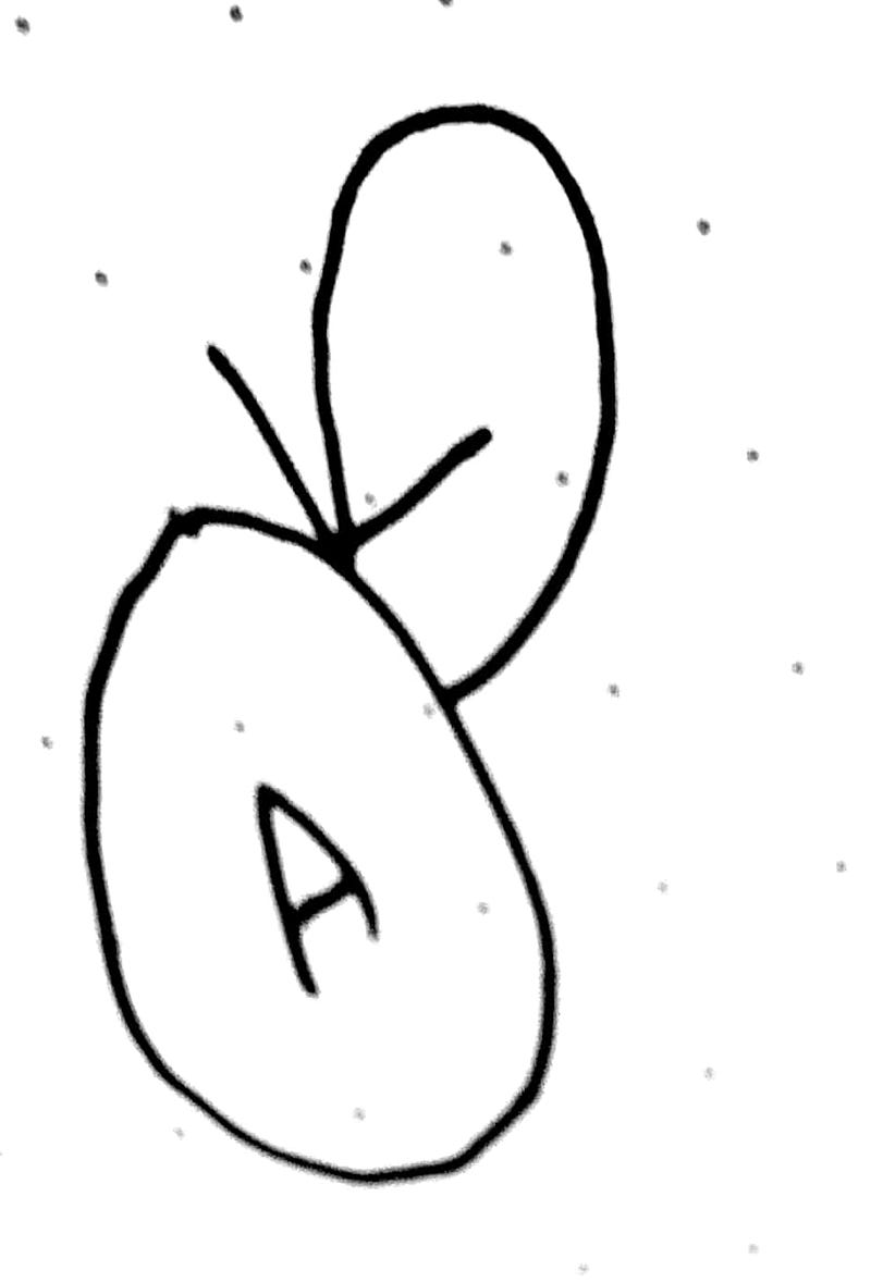
And this is not a simple graph, because a vertex exists with no edges connecting to it:
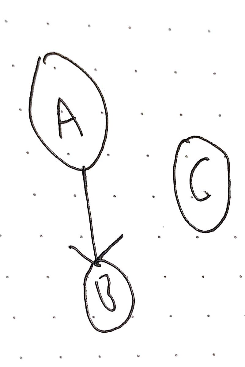
This is a simple graph:
Multi Graph
A multi graph allows more than one edge between two vertices:
More on Undirected Graphs and Terminology
In an undirected graph, G, suppose that e = {u, v} is an edge of G
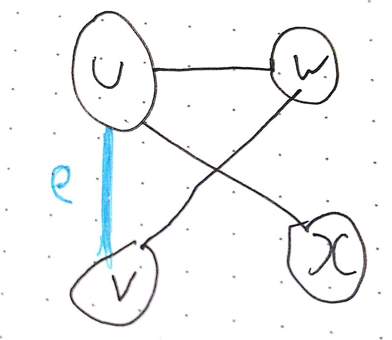
u and v are said to be adjacent and are called neighbours of each other
e is said to be incident with u and v
u and v are called endpoints of e
e is said to connect u and v
The degree of a vertex is how many edges are connected to it.
The degree of the graph is the maximum edges connected to a particular vertex. In this graph the degree is 3, since vertex u has degree 3 and is the largest degree in the graph.
Matrix Representation of Graphs
An undirected graph can be represented by an adjacency matrix.
A matrix is like a vector or a set, it’s a storage unit to store numbers in it.
An adjacency matrix, M, for a simple undirected graph with n vertices is called an n x n matrix.
In this matrix if vertex i and vertex j are adjacent (neighbours) then you can represent this on the matrix with the number 1.
If they are not, use the number 0.
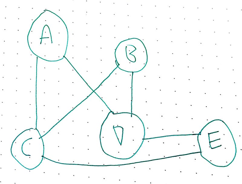
To represent this in a matrix, we can do the following:
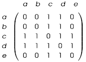
Notice how the diagonal is 0’s and if you take half of the upper triangle it matches the bottom half.
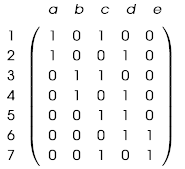
An incident matrix is an m x n matrix where m is the number of edges in the graph.
For this graph again:

We can use this incidence matrix to represent it:
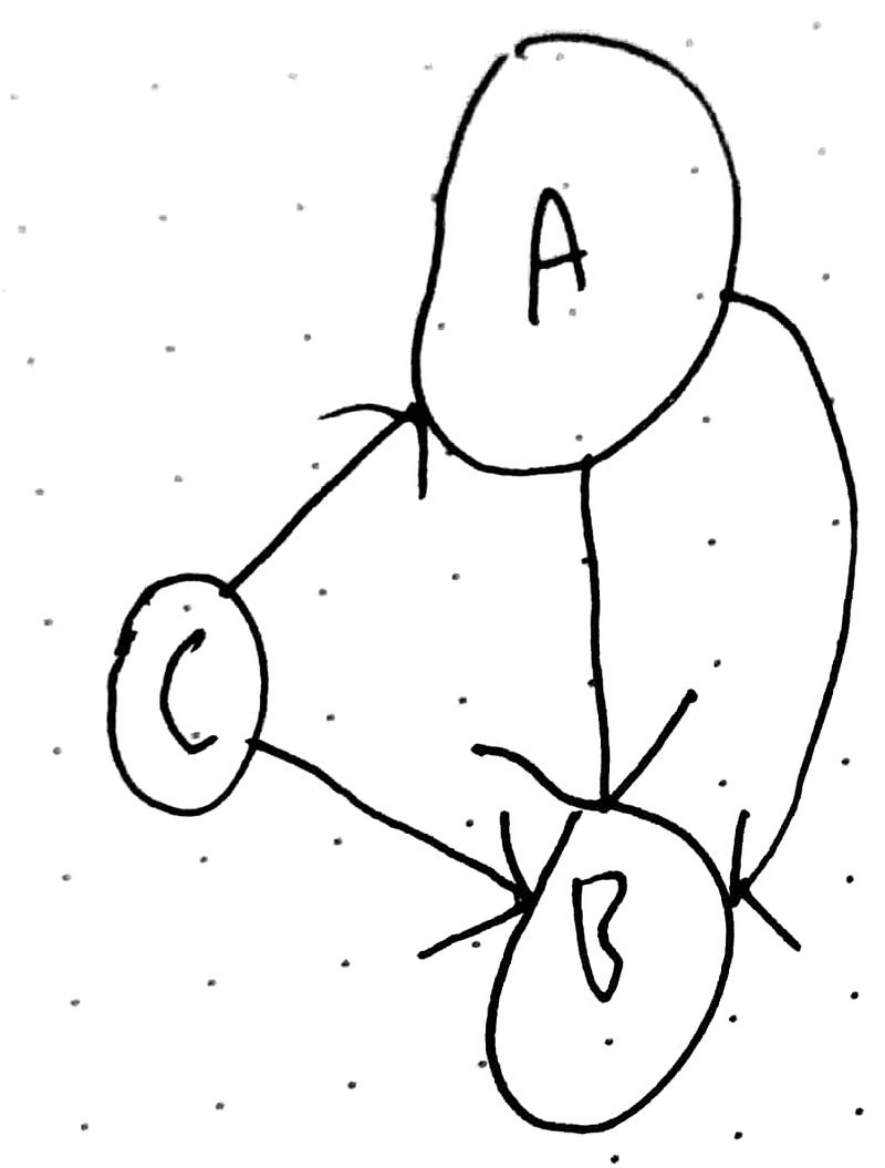
More on Directed Graphs
An in-degree of a vertex, v, is the number of edges leading to v.
An out-degree of a vertex, v, is the number of edges leading away from v.
The in-degree is the same as the out-degree. It’s also the same as the number of edges.
in degree sum = out degree sum
Because this is an **undirected **graph, the in degree and out degree have to be the same for each vertex.
If the total sum of all in degrees does not match the total sum of all out degrees then it is not a tree.
If you have 2 out-degrees and 1 in-degree it is not a tree since there is an edge either travelling nowhere or travelling to the same node twice.
A directed graph can be represented by an adjacency matrix or an incidence matrix.
Adjacency Matrix
An adjacency matrix, M, for a directed graph with n vertices is called an n x n matrix.
- M(i, j) is equal to 1 if (i, j) has an edge from i to j
- M(i, j) is otherwise 0.
An adjacency list is where each vertex, u, has a list of vertices pointed to by an edge leading away from u.
This is really nothing different from what we saw earlier.
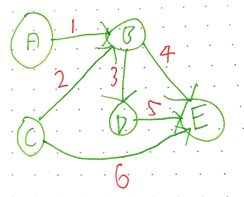
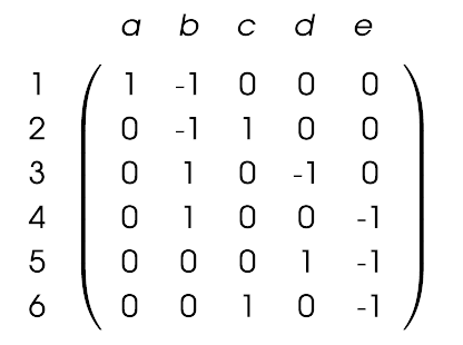
Incidence Matrix
An incidence matrix for a directed graph with n vertices and m edges is an m x n matrix.
These are the basic rules:
- M(i, j) = 1 if edge i is leading away from vertex j (leaving)
- M(i, j) = -1 if edge i is leading to vertex j (into)
- M(i, j) = 0 otherwise
Incidence list is a list where each vertex, u, has a list of vertices pointed to by an edge leading away from u.
Circuits
A circuit, a path, a cycle are all sequences of vertices and edges.
They all have rules and properties which make them special, these are:
- Cycle: Vertices cannot repeat. Edges cannot repeat.
- Walk: Vertices may repeat. Edges may repeat.
- Circuit: Vertices may repeat. Edges cannot repeat.
Normally a circuit is defined as a path from vertex a, back to vertex a.
A simple circuit visits an edge at most once (so never goes back to the same vertex).
An Euler circuit is a circuit visiting every edge exactly once (so can go back to the same vertex).
This is the exact same circuit Euler wanted to create on the Kronenbeig problem earlier. To cross every bridge (edge) exactly once, but allowing you to go to the vertexes (islands) as many times as you want.
The graph contains an Euler Circuit if and only if the degree of every vertex in the graph is even.
An Hamiltonian circuit (not named after Alexandria Hamilton) is a circuit containing every vertex of a graph, G, exactly once.
It does not matter in a Hamiltonian circuit whether or not you visit all of the edges.
Determining whether a graph contains a Hamiltonian circuit is an NP-hard problem. For information on NP-hardness click here.
Searching on Trees / Graphs
Okay, so we’ve met trees and graphs. But how do we search them? We can use some of these nifty search algorithms!
Breadth First Search
Breadth First Search (BFS) is a search algorithm developed by Konrad Zeus for his rejected PhD thesis in 1945. Breadth First Search searches all neighbours before it searches child nodes. In the below picture, once the start state (1) has been searched the states 2, 3, and 4 will then be searched.

The Breadth First Search Algorithm has a queue which is vital to how it works. Breadth first will first check whether the current node it is searching is the goal state or not. If it is not the goal state, it places all child nodes of the current node being searched into a queue. As an example assume the queue will look like [5, 6, 3, 4].
Because of the first in first out nature, the first ones added to the queue are the first ones out of the queue, so it would search in the order 4, 3, 6, 5.
Breadth first search searches in “levels”. It starts at level 1, [1], then goes down to level 2, [1:2, 1:3, 1:4].

When we look at a neighbour we need to see if it’s neighbours have been visited yet. In order to do this we need to “mark” the vertex to signify we haven’t looked at it yet.
Advantages
Breadth-first search is complete, as in it will always find a path and the shortest path to the goal, assuming the goal is at a finite depth.
Space and Time Complexity — A Quick Detour
Time complexity is how long it takes the algorithm to run given an input, usually denoted in Big O notation. Space complexity is how much the algorithm takes up in memory. Although this depends on the hardware factors, just like with Big O notation we can use a notation to represent how much space it’ll take up.
Consider a theoretical tree where node state has b successors. The root of the search tree generates b nodes and the second level of the search tree generates b² nodes. Each level generates b more nodes, yielding b^n (b to the power of n) nodes where n is the level the search tree is on. So the time complexity is $$b^n$$.
The space complexity of this is b^d.
You may notice this looks different from Big O notation, well, for some reason a lot of AI researchers use this notation. In big O the space and time complexity is:
O(|v|)
Where |v| is the number of nodes.
I believe this notation is used because it is the notation used in the book “Artificial Intelligence: A Modern Approach” by Russel and Norvig and because this book is the book on Artificial Intelligence everyone uses their notation.
b is the branching factor of the tree. d is the shallowest goal node (the lowest level at which a node is a goal for a given search problem) m is the maximum length of any path in the state space.
Disadvantages
Breadth First Search is very, very slow and requires a lot of memory, however, on a smaller graph / tree it is efficient.
Depth First Search
Depth First Search expands the deepest node in the current frontier first. Depth first search goes immediately to the deepest possible point of the search tree until there are no sucessors.
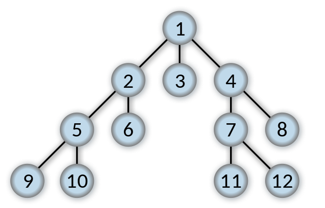
In this example, Depth First Search will go straight to 9, then 10 and then to 6.
Whereas Breadth First search uses a first in first out (FIFO) queue Depth First uses a a Last in Last out queue (LIFO). A LIFO queue means that the most recently generated node is chosen for expansion. The most recently generated node must be the deepest possible unexpanded node because it is deeper than its parent node.
If Depth First Search is used on a graph which avoids repeated states and redundant paths then it will find its goal in a finite number of states. If however it is used on a search tree then it will expand forever, in other words depth first search is not complete within search trees.
Depth first search will not find the optimal path.
The time complexity of DFS is 1+ b² + b³ + … +b^m
The advantage of DFS over BFS is the space complexity. Once a path has been fully explored it can be removed from memory, so DFS only needs to store the root node, all the children of the root node and where it currently is. DFS requires space complexity of bm where b is the branching factor and m is the longest path in the graph.