What is a decision tree in machine learning?

Decision trees, one of the simplest and yet most useful Machine Learning structures. Decision trees, as the name implies, are trees of decisions.

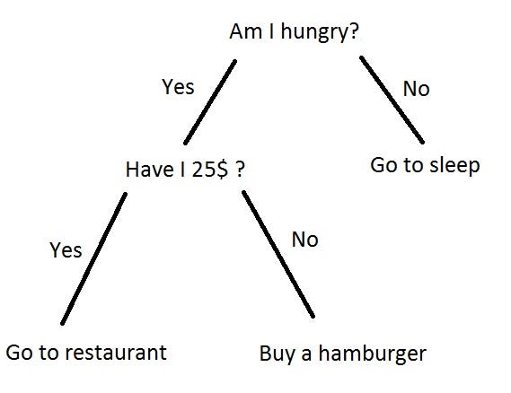
Taken from here You have a question, usually a yes or no (binary; 2 options) question with two branches (yes and no) leading out of the tree. You can get more options than 2, but for this article, we’re only using 2 options.

Trees are weird in computer science. Instead of growing from a root upwards, they grow downwards. Think of it as an upside down tree.

The top-most item, in this example, “Am I hungry?” is called the root. It’s where everything starts from. ***Branches ***are what we call each line. A ***leaf ***is everything that isn’t the root or a branch.

Trees are important in machine learning as not only do they let us visualise an algorithm, but they are a type of machine learning. Take this algorithm as an example.

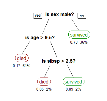
Taken from here This algorithm predicts the probability that a passenger will survive on the Titanic.

“sibsp” is the number of spouses or siblings aboard the ship. The figures under each leaf show the probability of survival.

With machine learning trees, the bold text is a condition. It’s not data, it’s a question. The branches are still called branches. The leaves are “decisions”. The tree has decided whether someone would have survived or died.

This type of tree is a **classification **tree. I talk more about classification here. In short; we want to classify each person on the ship as more likely to die or to have survived.

In real life, decision trees aren’t always as easy. Take a look at this photo, and brace yourself. I’ll try to describe as much of it as I can.

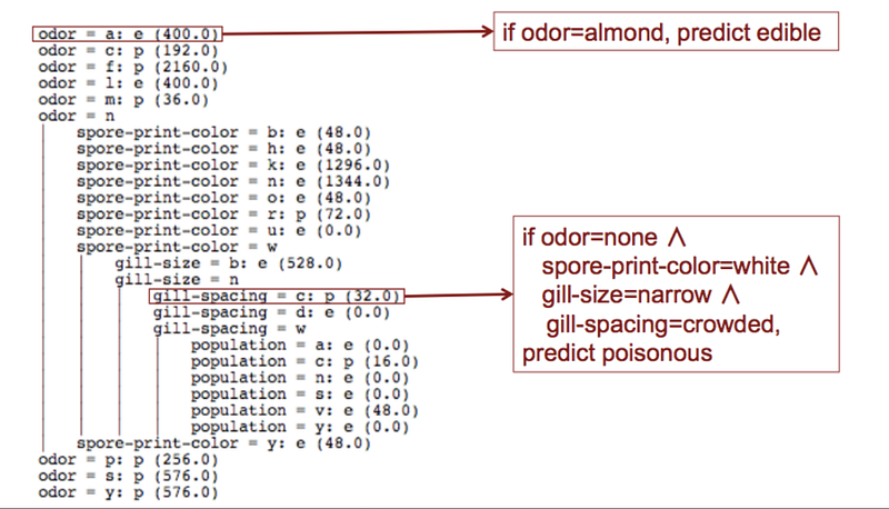
😴 — Me when I have to look at this image This is a decision tree. It wants to answer the question “can I eat this mushroom?”

Taken from here Given an image of a mushroom (like on the left) we want to find out if it’s edible.

You see those things at the top which look like variable assignments? Those are if statements. Let’s take a look at one of those.

“odor = a: e (400.0)”

If the smell (odor) of the mushroom is “a” for almond, then it is edible (e) and we are 400.0 points confident that it is edible. Each of these statements is a feature.

Features are just attributes of an object. The features of a bike are: it has wheels, it has handlebars etc.

We do this on and on until we reach a point where the odor is neutral (n) at which point we start to check more **features **of the mushroom.

Making decision trees using a formal language

Okay, We can draw them but how do we write decision trees? There’s a nice notation for that.

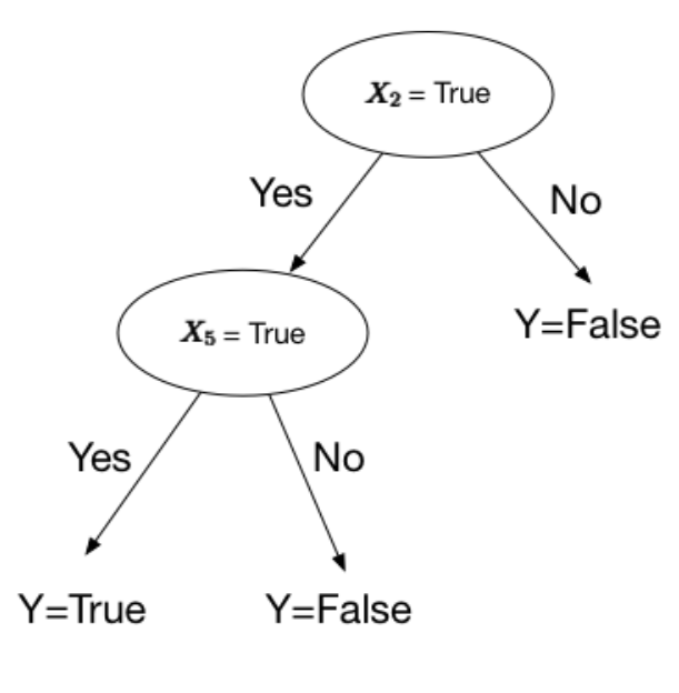
Let’s jump right into an example.

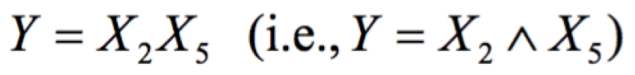
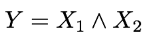
Sorry for the blurry formula. It’s a problem with screen shotting LaTeX 😢 The fancy little “^” means “and”. It’s some fancy mathematical notation. For more notation like this, check out this other article I wrote. In this notation, when we don’t see anything connecting 2 items (like x2 and x5) we assume it is “and”. We want a decision tree that returns **True **when both *x2 *and x5 are true.

Okay, let’s see another one.

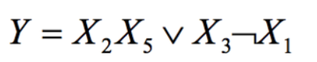
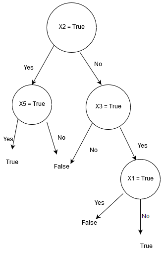
This one features a lot more logic symbols. You might want to check out this other article I wrote. Okay, the “∨” symbol means “or” and the “¬” means “not”.

Notice how the X1 decision becomes True if X1 is **not **true. This is because of the “not” symbol before it in the formal notation.

Splitting candidates in the tree

Decision trees are made by taking data from the root node and splitting the data into parts.

Taken from here Taking the Titanic example from earlier, we split the data so that it makes the most sense and is in alignment with the data we have.

One of the problems with decision trees is the question “what is the best way to split the data?” Sometimes you’ll instinctively know, other times you’ll need an algorithm

We want to design a function which when given a dataset will split the data accordingly.

If we have numerical features we can split it based on the data we see. There are many different ways of splitting. We can sort all the values in the dataset and decide the split thresholds between instances of different classes. We can also cut them straight down the middle. There are too many splitting algorithms to discuss here. So instead we’ll go through a simple algorithm.(1, a), (2, b), (1, c), (0, b), (3, b)

So we have 3 classes (a, b, c). The first thing we do is put them into different categories.

{(0, b)}, {(1, a), (1, c)}, {(2, b)}, {(3, b)}

Now we have 4 different sets. For more on set theory, click here.

Let’s just pick some arbitrary numbers here. We’ll split them like so:

Split 1 <= 0.5
Split 2 <= 1.5 but > 0.5
Split 3 > 1.5

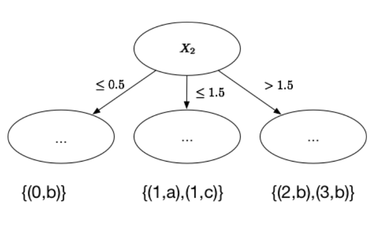
We now have a decision tree split up. If we didn’t split the data up, the tree wouldn’t look much like a tree. Imagine what the tree might look like if our split was “all data less than 3”. Everything would be there! It wouldn’t be very tree-like.

Occam’s razor

Image of William of Ockham, from here. Occam’s razor is a philosophy attributed to William of Ockham in the 14th century. In short, the quote is:

“When you have two competing theories that make exactly the same predictions, the simpler one is the better one.”

We can use this principle in machine learning, especially when deciding when to split up decision trees.

“The simplest tree that classifies the training instances accurcately will work well on previously unseen instances.”

The simplest tree will often be the best tree, so long as all other possible trees make the same results.

Finding the best splitsGif from Giphy. Sometimes, the subject you’re teaching is just plain old boring. Gif provided to try to alleviate the boredom.

Trying to find and return the smallest possible decision tree that accurately classifies the training set is very very hard. In fact, it’s an NP-hard problem.

Instead, we’ll try to approximate the best result instead of getting the best result. We’re going to talk a lot about probability and statistics, if you want to know more about probability and statistics click here.

What we want is information that explicitly splits the data into two. We don’t want something that can include both male and females, we want purity. One singular class for each split.

This measure of purity is called information. It represents the expected amount of information that would be needed to specify whether a new instance should be classified as the left or right split.

To find the best splits, we must first learn a few interesting things.

Expected Value

This part talks about random variables. For more on random variables, check out this article on statistics & probability I wrote.

The expected value is exactly what it sounds like, what do you expect the value to be? You can use this to work out the average score of a dice roll over 6 rolls, or anything relating to probability where it has a value property.

Suppose we’re counting types of bikes, and we have 4 bikes. We assign a code to each bike like so:

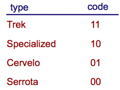
For every bike, we give it a number. For every coding, we can see we use 2 bits. Either 0 or 1. For the expected value, not only do we need the value for the variable but the probability. Each bike has equal probability. So each bike has a 25% chance of appearing.

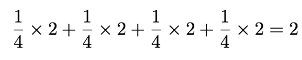
Calculating the expected value we multiply the probability by 2 bits, which gets us:

What if the probability wasn’t equal?

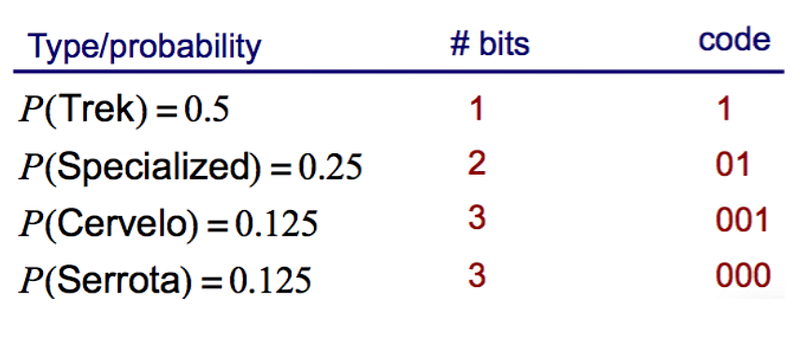
What we need to do is to multiply the number of bits by the probability

Entropy

This measure of purity is called the information. It represents the expected amount of information that would be needed to specify whether a new instance (first-name) should be classified as male or female, given the example that reached the node. We calculate it based on the number of male and female classes at the node.

Remember earlier when we talked about purity? Entropy is a measure of impurity. It’s how uncertain something is. The formula for entropy is:

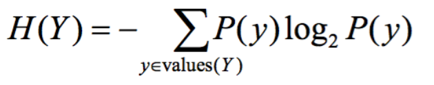
Entropy is trying to give a number to how uncertain something is.

You can also have conditional entropy, which looks like this:

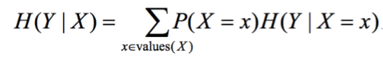
Information Gain Example

Let’s show this using an example.

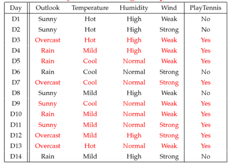
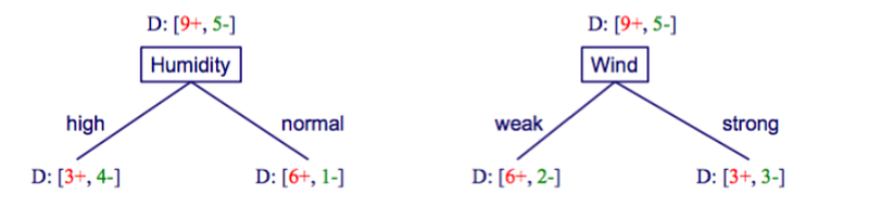
What’s the information gain of splitting on Humidity?

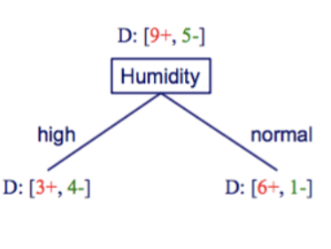
An example of splitting on humidity We have 9+ and 5-. What does that mean? That means in the table we have 9 features where data is positive and 5 where it’s no. So go down the PlayTennis table and count 9 times for positive (Yes) and 5 times for negative (No).

Now we want to find out the information gain of humidity. If humidity is high, we look at the data and count how many yes’s for humidity high. So when humidity is high, we have 3+ and 4-. 3 positives and 4 negatives.

D indicates the specific sample, D.

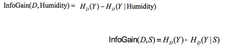
The information gain is the gap between uncertainty. We have 14 sets of data in total, The denominator is always 14. Now we just calculate them using the formula. The information gain of playing tennis (yes) when the humidity is high is:

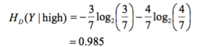
3 yes’s and 4 no’s And the information gain of playing tennis when the humidity is normal is:

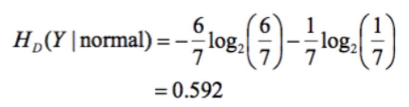
6 yes’s and 1 no. This isn’t how likely something is to happen, it’s just how much information we gain from this. We use information gain when we want to split something. In the below example we want to find out whether it is better to split on humidity or wind.

Now we know what the information gain on each split is using entropy, we apply the information gain formula.

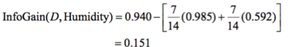
The information gain on splitting by humidity amongst our sample, D, is 0.151.

If we use the same formula for entropy in the wind part, we get these results:

And if we put them into the information gain formula we get:

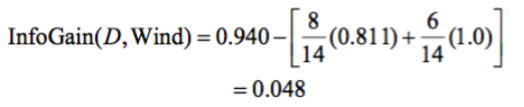
It is better to split on humidity rather than wind as humidity has a higher information gain.

Definition of accuracy

What we want to do is to check how accurate a machine learning model is.

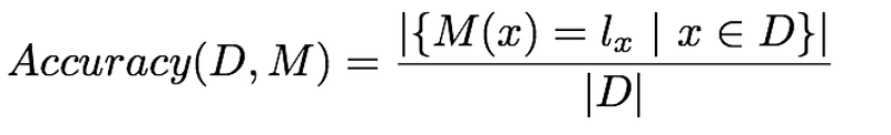
M(x) means given a sample, X, we give the predicted classification. The label. lx is actually the true label. So this sample has already been labeled so we know the true label. This set of samples shows that these are correctly labeled.

What we do is feed the algorithm a sample set where we already know the classification of every single item in that sample set. We then measure how many times the machine learning algorithm was right.

Overfitting with noisy data

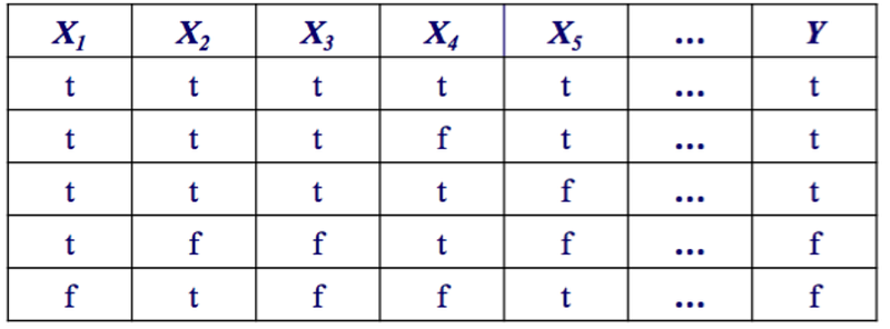
Look at the below example. We have this formula and noisy data.

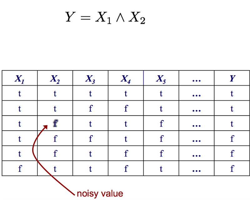
Noisy data means that the data isn’t correct. Our formula is X1 and X2 = True. Our noisy data is True and False = True, which is wrong.

The x3, x4, x5 are all additional features. We don’t care about them, but this is just an example to show that sometimes we have many additional features in a machine learning model which we don’t care about.

We build a decision tree that can match the training data perfectly.

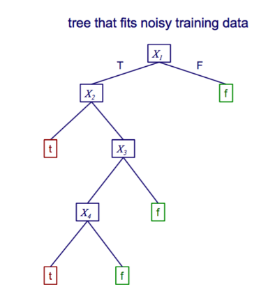
The accuracy is

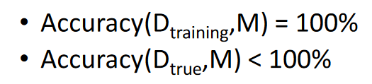
The problem is that it matches the training data perfectly, 100% but because of the noisy data it doesn’t perform very well on the true data. That one small error makes a larger decision tree and causes it to not perform as well in the real world.

If we build a decision tree that works well with the true data, we’ll get this:

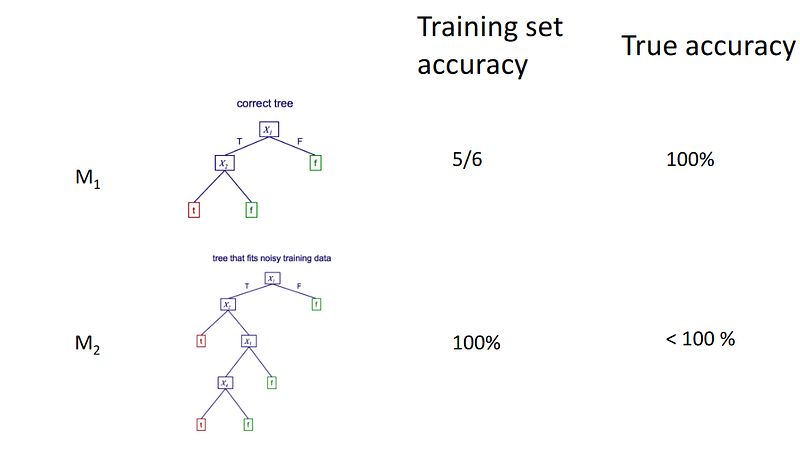
Even though it performs worse in the training set, due to not worrying about noisy data it performs perfectly with real-world data.

Let’s see another example of overfitting.

Overfitting with noise-free data

Here are the probabilities for each one:

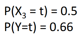
There’s a 50% chance that the resultant,* x3*, is True. There’s a 0.66% chance that the resultant, *Y*, is True.

For our first model let’s have a quick look.

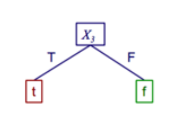
The accuracy is:

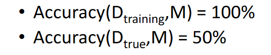
It’s good on training data, but on real world data (D_true) it doesn’t perform as well. From this, we can tell that overfitting has occurred.

Preventing overfitting

The reason for overfitting is because the training model is trying to fit as well as possible over the training data, even if there is noise within the data. The first suggestion is to try and reduce noise in your data.

Another possibility is that there is no noise, but the training data is small resulting in a difference from the true sample. More data would work.

It’s hard to give an exact idea of how to prevent overfitting as it differs from model to model.