Greedy Algorithms In Python


Greedy algorithms aim to make the optimal choice at that given moment. Each step it chooses the optimal choice, without knowing the future. It attempts to find the globally optimal way to solve the entire problem using this method.
Why Are Greedy Algorithms Called Greedy?
We call algorithms greedy when they utilise the greedy property. The greedy property is:
At that exact moment in time, what is the optimal choice to make?
Greedy algorithms are greedy. They do not look into the future to decide the global optimal solution. They are only concerned with the optimal solution locally. This means that the overall optimal solution may differ from the solution the algorithm chooses.
They never look backwards at what they’ve done to see if they could optimise globally. This is the main difference between Greedy and Dynamic Programming.
To be extra clear, one of the most Googled questions about greedy algorithms is:
“What problem-solving strategies don’t guarantee solutions but make efficient use of time?”
The answer is “Greedy algorithms”. They don’t guarantee solutions but are very time efficient. However, in the next section, we’ll learn that sometimes Greedy solutions give us the optimal solutions.
What Are Greedy Algorithms Used For?
Greedy algorithms are quick. A lot faster than the two other alternatives (Divide & Conquer, and Dynamic Programming). They’re used because they’re fast.
Sometimes, Greedy algorithms give the global optimal solution every time. Some of these algorithms are:
These algorithms are Greedy, and their Greedy solution gives the optimal solution.
We’re going to explore greedy algorithms using examples, and learning how it all works.
How Do I Create a Greedy Algorithm?
Your algorithm needs to follow this property:
At that exact moment in time, what is the optimal choice to make?
And that’s it. There isn’t much to it. Greedy algorithms are easier to code than Divide & Conquer or Dynamic Programming.
Counting Change Using Greedy
Imagine you’re a vending machine. Someone gives you £1 and buys a drink for £0.70p. There’s no 30p coin in pound sterling, how do you calculate how much change to return?
For reference, this is the denomination of each coin in the UK:
1p, 2p, 5p, 10p, 20p, 50p, £1
The greedy algorithm starts from the highest denomination and works backwards. Our algorithm starts at £1. £1 is more than 30p, so it can’t use it. It does this for 50p. It reaches 20p. 20p < 30p, so it takes 1 20p.
The algorithm needs to return a change of 10p. It tries 20p again, but 20p > 10p. It next goes to 10p. It chooses 1 10p, and now our return is 0 we stop the algorithm.
We return 1x20p and 1x10p.
This algorithm works well in real life. Let’s use another example, this time we have the denomination next to how many of that coin is in the machine, (denomination, how many).
(1p, 10), (2p, 3), (5p, 1), (10p, 0), (20p, 1p), (50p, 19p), (100p, 16)
The algorithm is asked to return a change of 30p again. 100p (£1) is no. Same for 50. 20p, we can do that. We pick 1x 20p. We now need to return 10p. 20p has run out, so we move down 1.
10p has run out, so we move down 1.
We have 5p, so we choose 1x5p. We now need to return 5p. 5p has run out, so we move down one.
We choose 1 2p coin. We now need to return 3p. We choose another 2p coin. We now need to return 1p. We move down one.
We choose 1x 1p coin.
Our algorithm selected these coins to return as change:
# (value, how many we return as change)
(10, 1)
(5, 1)
(2, 2)
(1, 1)
Let’s code something. First, we need to define the problem. We’ll start with the denominations.
denominations = [1, 2, 5, 10, 20, 50, 100]
# 100p is £1
Now onto the core function. Given denominations and an amount to give change, we want to return a list of how many times that coin was returned.
If our denominations list is as above, [6, 3, 0, 0, 0, 0, 0] represents taking 6x1p coins and 3x2p coins, but 0 of all other coins.
denominations = [1, 2, 5, 10, 20, 50, 100]
# 100p is £1

def returnChange(change, denominations):
    toGiveBack = [0] * len(denominations)
    for pos, coin in reversed(list(enumerate(denominations))):
We create a list, the size of denominations long and fill it with 0’s.
We want to loop backwards, from largest to smallest. Reversed(x) reverses x and lets us loop backwards. Enumerate means “for loop through this list, but keep the position in another variable”. In our example when we start the loop. coin = 100 and pos = 6.
Our next step is choosing a coin for as long as we can use that coin. If we need to give change = 40 we want our algorithm to choose 20, then 20 again until it can no longer use 20. We do this using a for loop.
denominations = [1, 2, 5, 10, 20, 50, 100]
# 100p is £1

def returnChange(change, denominations):
    # makes a list size of length denominations filled with 0
    toGiveBack = [0] * len(denominations)

    # goes backwards through denominations list
    # and also keeps track of the counter, pos.
    for pos, coin in enumerate(reversed(denominations)):
        # while we can still use coin, use it until we can't
        while coin <= change:
While the coin can still fit into change, add that coin to our return list, toGiveBack and remove it from change.
denominations = [1, 2, 5, 10, 20, 50, 100]
# 100p is £1

def returnChange(change, denominations):
    # makes a list size of length denominations filled with 0
    toGiveBack = [0] * len(denominations)

    # goes backwards through denominations list
    # and also keeps track of the counter, pos.
    for pos, coin in enumerate(reversed(denominations)):
        # while we can still use coin, use it until we can't
        while coin <= change:
            change = change - coin
            toGiveBack[pos] += 1
    return(toGiveBack)

print(returnChange(30, denominations))
# returns [0, 0, 0, 1, 1, 0, 0]
# 1x 10p, 1x 20p
The runtime of this algorithm is dominated by the 2 loops, thus it is O(n2)O(n2).
Is Greedy Optimal? Does Greedy Always Work?
It is optimal locally, but sometimes it isn’t optimal globally. In the change-giving algorithm, we can force a point at which it isn’t optimal globally.
The algorithm for doing this is:
- Pick 3 denominations of coins. 1p, x, and less than 2x but more than x.
We’ll pick 1, 15, 25.
- Ask for a change of 2 * second denomination (15)
We’ll ask for a change of 30. Now, let’s see what our Greedy algorithm does.
[5, 0, 1]
It choses 1x 25p, and 5x 1p. The optimal solution is 2x 15p.
Our Greedy algorithm failed because it didn’t look at 15p. It looked at 25p and thought “Yup, that fits. Let’s take it.”
It then looked at 15p and thought “That doesn’t fit, let’s move on”.
This is an example of where Greedy Algorithms fail.
To get around this, you would either have to create currency where this doesn’t work or brute-force the solution. Or use Dynamic Programming.
Dijkstra’s Algorithm
Dijkstra’s algorithm finds the shortest path from a node to every other node in the graph. In our example, we’ll be using a weighted directed graph. Each edge has a direction, and each edge has a weight.
Dijkstra’s algorithm has many uses. It can be very useful within road networks where you need to find the fastest route to a place. We also use the algorithm for:
The algorithm follows these rules:
- Every time we want to visit a new node, we will choose the node with the smallest known distance.
- Once we’ve moved to the node, we check each of its neighbouring nodes. We calculate the distance from the neighbouring nodes to the root nodes by summing the cost of the edges that lead to that new node.
- If the distance to a node is less than a known distance, we’ll update the shortest distance.
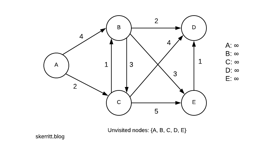
Our first step is to pick the starting node. Let’s choose A. All the distances start at infinity, as we don’t know their distance until we reach a node that knows the distance.
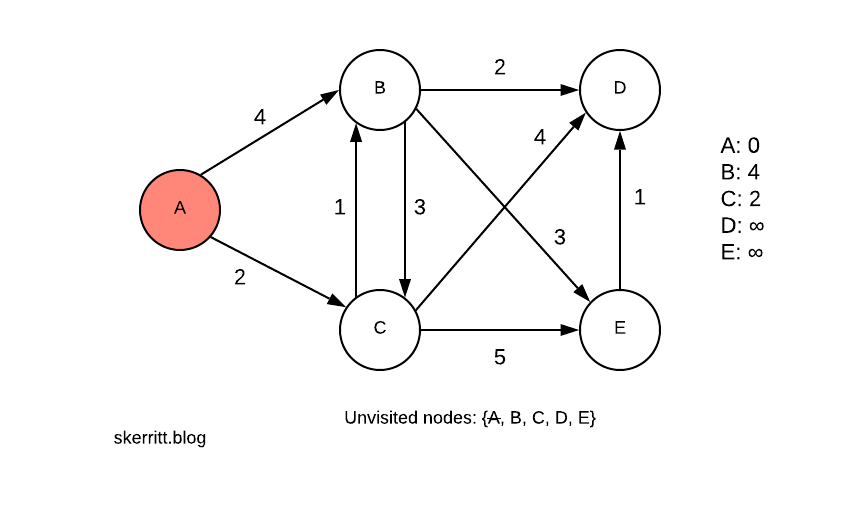
We mark off A on our unvisited nodes list. The distance from A to A is 0. The distance from A to B is 4. The distance from A to C is 2. We updated our distance listing on the right-hand side.
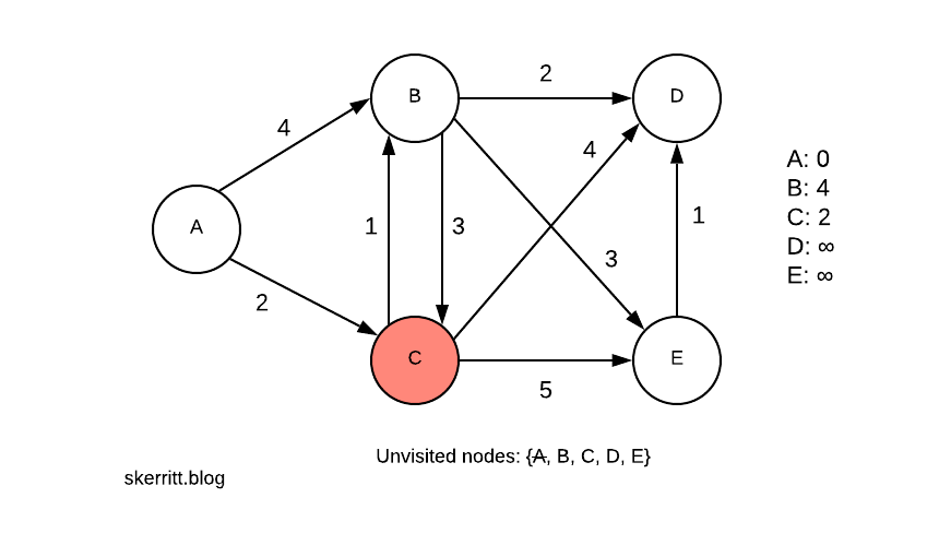
We pick the smallest edge where the vertex hasn’t been chosen. The smallest edge is A -> C, and we haven’t chosen C yet. We visit C.
Notice how we’re picking the smallest distance from our current node to a node we haven’t visited yet. We’re being greedy. Here, the greedy method is the global optimal solution.
We can get to B from C. We now need to pick a minimum min(4, 2+1)=3.
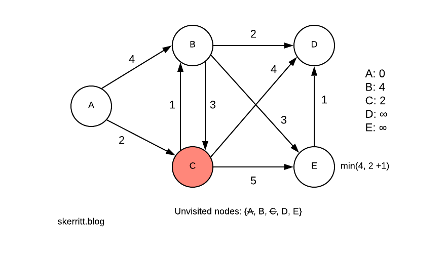
Since A -> C -> B is smaller than A -> B, we update B with this information. We then add in the distances from the other nodes we can now reach.

Our next smallest vertex with a node we haven’t visited yet is B, with 3. We visit B.
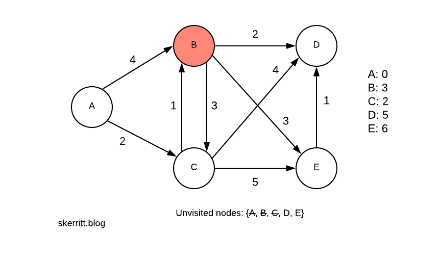
We do the same for B. Then we pick the smallest vertex we haven’t visited yet, D.
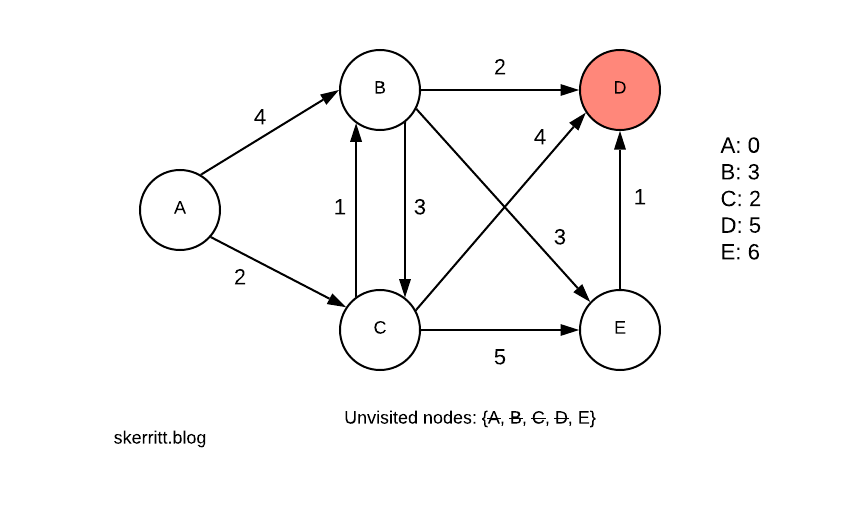
We don’t update any of the distances this time. Our last node is then E.
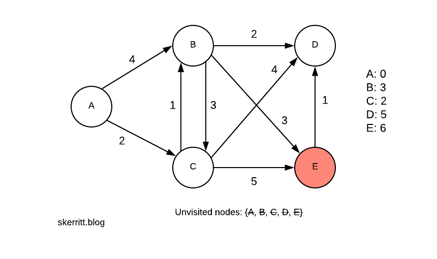
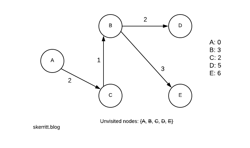
There are no updates again. To find the shortest path from A to the other nodes, we walk back through our graph.
We pick A first, C second, B third. If you need to create the shortest path from A to every other node as a graph, you can run this algorithm using a table on the right-hand side.
| Dijkstra's Table | ||
|---|---|---|
| Node | Distance from A | Previous node |
| A | 0 | N/A |
| B | 3 | C |
| C | 2 | A |
| D | 5 | B |
| E | 6 | B |
Using this table it is easy to draw out the shortest distance from A to every other node in the graph:
Minimum Spanning Trees Using Prim’s Algorithm
Prim’s algorithm is a greedy algorithm that finds a minimum spanning tree for a weighted undirected graph. It finds the optimal route from every node to every other node in the tree.
With a small change to Dijkstra’s algorithm, we can build a new algorithm - Prim’s algorithm!
We informally describe the algorithm as:
- Create a new tree with a single vertex (chosen randomly)
- Of all the edges not yet in the new tree, find the minimum weighted edge and transfer it to the new tree
- Repeat step 2 until all vertices are in the tree
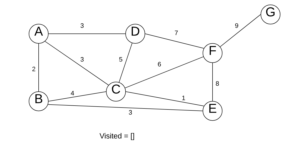
We have this graph.
Our next step is to pick an arbitrary node.

We pick the node A. We then examine all the edges connecting A to other vertices. Prim’s algorithm is greedy. That means it picks the shortest edge that connects to an unvisited vertex.
In our example, it picks B.
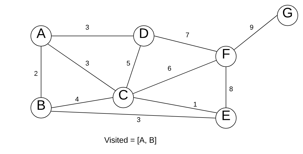
We now look at all nodes reachable from A and B. This is the distinction between Dijkstra’s and Prim’s. With Dijkstra’s, we’re looking for a path from 1 node to a certain other node (nodes that have not been visited). With Prim’s, we want the minimum spanning tree.
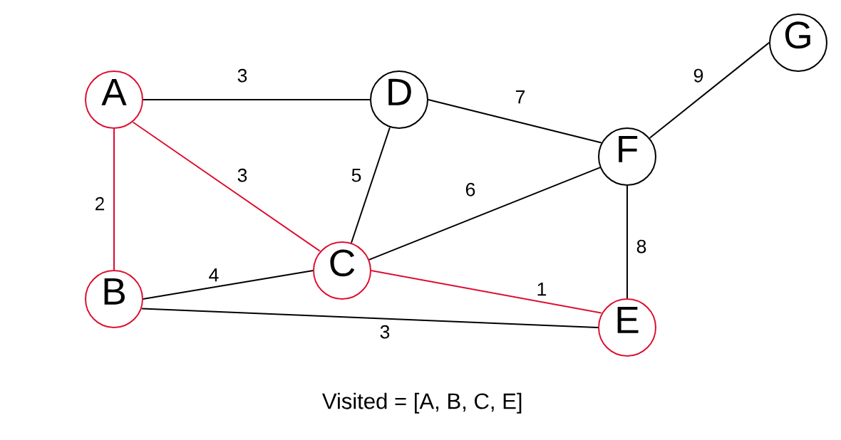
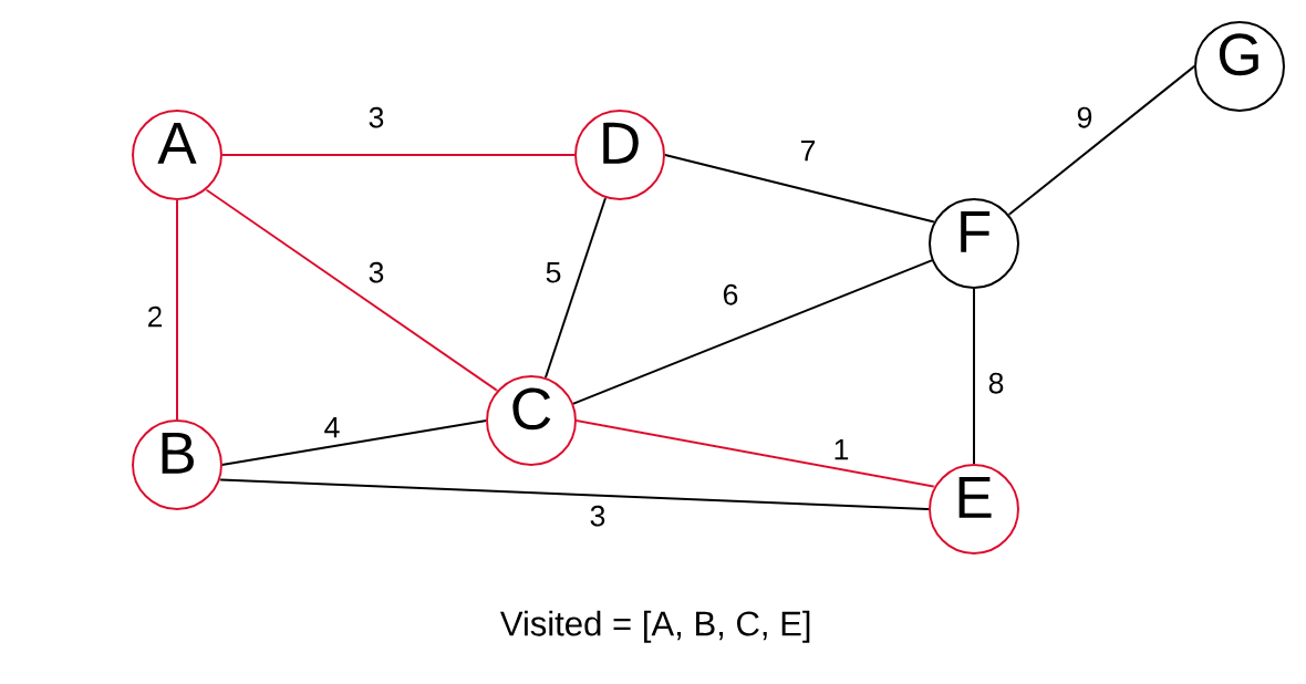
We have 3 edges with equal weights of 3. We pick 1 randomly.
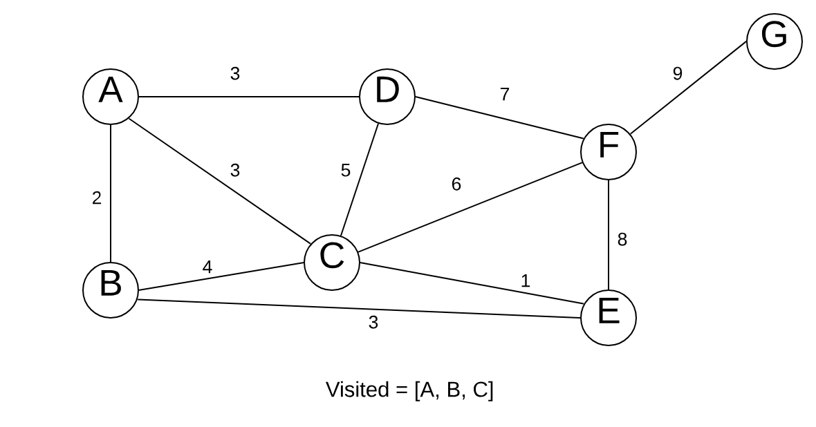
It is helpful to highlight our graph as we go along because it makes it easier to create the minimum spanning tree.
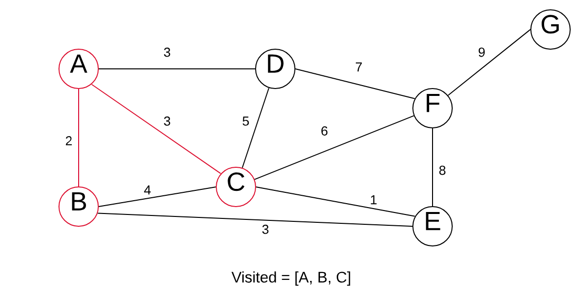
Now we look at all edges of A, B, and C. The shortest edge is C > E with a weight of 1.
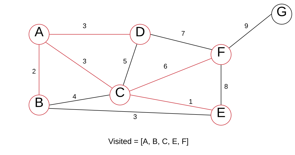
And we repeat:
The edge B > E with a weight of 3 is the smallest edge. However, both vertices are always in our VISITED list. Meaning we do not pick this edge. We instead choose C > F, as we have not visited
The only node left is G, so let’s visit it.
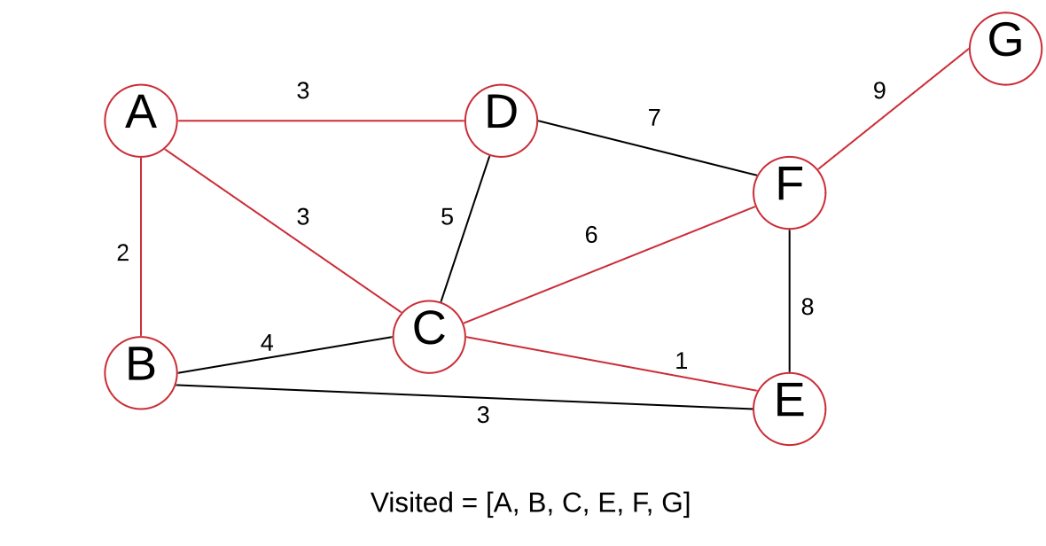
Note that if the edge weights are distinct, the minimum spanning tree is unique.
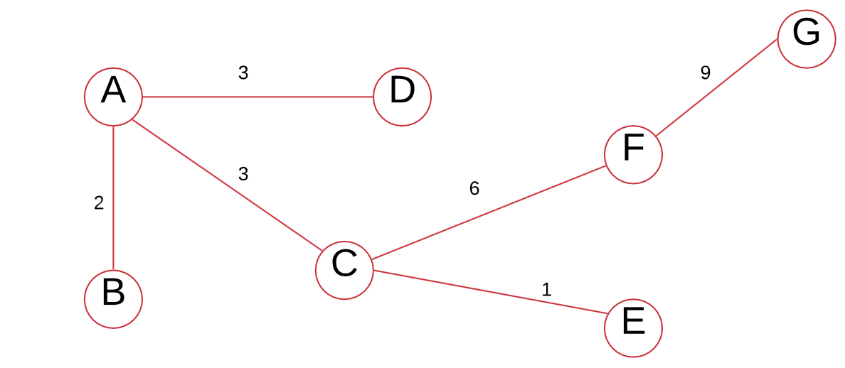
We can add the edge weights to get the minimum spanning tree’s total edge weight:
$$2+3+3+1+6+9=24$$
Fractional Knapsack Problem Using Greedy Algorithm
Imagine you are a thief. You break into the house of Judy Holliday - 1951 Oscar winner for Best Actress. Judy is a hoarder of gems. Judy’s house is lined to the brim with gems.
You brought with you a bag - a knapsack if you will. This bag has a weight of 7. You happened to have a listing of Judy’s items, from some insurance paper. The items read as:
| Judy's Items | ||
|---|---|---|
| Name | Value | Weight |
| Diamonds | 16 | 5 |
| Francium | 3 | 1 |
| Sapphire | 6 | 2 |
| Emerald | 2 | 1 |
The first step to solving the fractional knapsack problem is to calculate \(\frac{value}{weight}\) for each item.
Judy's Items | |||
|---|---|---|---|
| Name | Value | Weight | Value / weight |
| Diamonds | 16 | 5 | 3.2 |
| Francium | 3 | 1 | 3 |
| Sapphire | 6 | 2 | 3 |
| Emerald | 2 | 1 | 2 |
And now we greedily select the largest ones. To do this, we can sort them according to \(\frac{value}{weight}\)
in descending order. Luckily for us, they are already sorted. The largest one is 3.2.
knapsack value = 16
knapsack total weight = 5 (out of 7)
Then we select Francium (I know it’s not a gem, but Judy is a bit strange 😉)
knapsack value = 19
knapsack weight = 6
Now, we add Sapphire. But if we add Sapphire, our total weight will come to 8.
In the fractional knapsack problem, we can cut items up to take fractions of them. We have a weight of 1 left in the bag. Our sapphire has weight 2. We calculate the ratio of:
$$\frac{weight\;of\;knapsack\;left}{weight\;of\;item}$$
And then multiply this ratio by the value of the item to get how much value of that item we can take.
$$\frac{1}{2} * 6 = 3$$
knapsack value = 21
knapsack weight = 7
The greedy algorithm can optimally solve the fractional knapsack problem, but it cannot optimally solve the {0, 1} knapsack problem. In this problem instead of taking a fraction of an item, you either take it {1} or you don’t {0}. To solve this, you need to use Dynamic Programming.
The runtime for this algorithm is O(n log n). Calculating \(\frac{value}{weight}\) is O(1). Our main step is sorting from largest \(\frac{value}{weight}\), which takes O(n log n) time.
Greedy vs Divide & Conquer vs Dynamic Programming
| Greedy vs Divide & Conquer vs Dynamic Programming | ||
|---|---|---|
| Greedy | Divide & Conquer | Dynamic Programming |
| Optimises by making the best choice at the moment | Optimises by breaking down a subproblem into simpler versions of itself and using multi-threading & recursion to solve | Same as Divide and Conquer, but optimises by caching the answers to each subproblem as not to repeat the calculation twice. |
| Doesn't always find the optimal solution, but is very fast | Always finds the optimal solution, but is slower than Greedy | Always finds the optimal solution, but could be pointless on small datasets. |
| Requires almost no memory | Requires some memory to remember recursive calls | Requires a lot of memory for memoisation / tabulation |
To learn more about Divide & Conquer and Dynamic Programming, check out these 2 posts I wrote:
Conclusion
Greedy algorithms are very fast, but may not provide the optimal solution. They are also easier to code than their counterparts.